Case Study 3 • FSSgam.docs

Overview

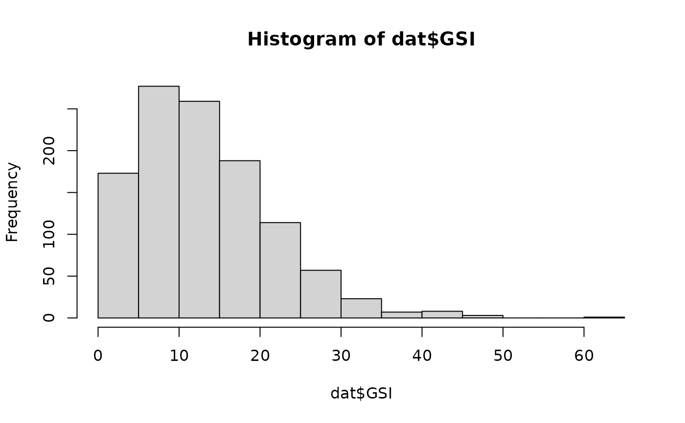
This case study examines reproductive patterns over multiple temporal scales in two tropical intertidal gastropods using full subsets Generalised Additive Models (GAMs). The response variable is gonadosomatic index (GSI), modelled using a Gamma distribution.

The example demonstrates how cyclic smoothers and factor interactions can be combined within the FSSgam framework to analyse lunar, semi‑lunar and seasonal reproductive patterns.

Background

Many marine invertebrates exhibit reproductive cycles across multiple temporal scales, including seasonal, lunar and semi‑lunar rhythms. These cycles are difficult to analyse using traditional categorical approaches because both seasonality and lunarity are inherently cyclic processes.

Generalised Additive Models (GAMs) provide a flexible framework for examining non‑linear, cyclic patterns and their interactions with biological factors such as sex and species. Here, GAMs with full subsets selection are used to disentangle monthly and lunar drivers of reproductive output in two common intertidal gastropods: Patelloida saccharina and Monodonta labio.

R packages

library(mgcv)
library(MuMIn)
library(FSSgam)
library(tidyverse)

Data preparation

Load the case study data and ensure year is treated as a factor.

dat <- case_study3 |> 
  mutate(year = factor(year))

Response variable distribution

hist(dat$GSI)

range(dat$GSI)

## [1]  0.6125574 60.9473024

GSI is a continuous, slightly right‑skewed variable without zeros, supporting the use of a Gamma distribution.

Predictor specification

Both lunar.date and month are entered into the model as continous cyclic smooths. This ensures that that end tails of the smooths meet smoothly. For example, this means that the estimate for Dec smoothly links to estimates from January, in the case of month.

Sex and Species are included as factors.

cyclic.vars <- c("lunar.date", "month")
cont.vars   <- c("lunar.date", "month")
factor.vars <- c("Sex", "Species")

Both month and lunar date are treated as cyclic continuous predictors, allowing smooth transitions at their boundaries.

Full subsets GAM analysis

GSI is modelled as a Gamma distribution.

Sex and Species are included as interaction terms with each other (via factor.factor.interactions = TRUE), and as interaction terms between the two smoothers (this is default behaviour for FSSgam, see ?generate.model.set).

Model assessment

Examine predictor correlations. This looks as would be expected. Note the function does estimate correlations between factors as well as continuous predictors. See ?generate.model.set for more details on how this is done.

model.set$predictor.correlations

##                lunar.date      month         Sex    Species Sex.I.Species
## lunar.date    1.000000000 0.03997010 0.002458829 0.03577236    0.03618006
## month         0.039970104 1.00000000 0.010673718 0.04418362    0.05979362
## Sex           0.002458829 0.01067372 1.000000000 0.04597970    0.99999995
## Species       0.035772358 0.04418362 0.045980185 1.00000000    0.99999995
## Sex.I.Species 0.036180060 0.05979362 0.707483898 0.70747167    1.00000000

Examine the model table. Note that the bet model includes all of the predictors, with interactions between lunar date and species, month and species, and an additive effect of Sex.

mod.table <- out.list$mod.data.out
mod.table <- mod.table[order(mod.table$AICc), ]

tab <- mod.table |>
  as_tibble() |> 
  select(modname, AICc, r2.vals, edf, delta.AICc, wi.AICc)

knitr::kable(
  tab,
  digits = 3,
  caption = "Model comparison summary based on AICc"
)

Model comparison summary based on AICc
modname	AICc	r2.vals	edf	delta.AICc	wi.AICc
lunar.date.by.Species+month.by.Species+Sex+Species	7233.999	0.276	13.96	0.000	0.998
lunar.date.by.Sex.I.Species+month.by.Sex.I.Species+Sex.I.Species	7246.967	0.273	23.26	12.968	0.002
lunar.date.by.Species+month.by.Species+Species	7296.470	0.228	12.88	62.471	0.000
lunar.date.by.Species+month+Sex+Species	7339.484	0.208	11.21	105.484	0.000
lunar.date+month.by.Species+Sex+Species	7342.382	0.224	11.25	108.383	0.000
lunar.date.by.Sex+month.by.Species+Sex+Species	7343.588	0.223	14.02	109.589	0.000
lunar.date.by.Species+month.by.Sex+Sex+Species	7344.032	0.207	13.50	110.033	0.000
lunar.date.by.Sex.I.Species+month+Sex.I.Species	7344.862	0.205	16.10	110.863	0.000
lunar.date+month.by.Sex.I.Species+Sex.I.Species	7348.601	0.222	16.58	114.602	0.000
lunar.date.by.Species+Sex+Species	7348.865	0.198	8.70	114.866	0.000
lunar.date.by.Sex.I.Species+Sex.I.Species	7354.790	0.194	13.49	120.791	0.000
month.by.Species+Sex+Species	7378.703	0.189	8.11	144.704	0.000
month.by.Sex.I.Species+Sex.I.Species	7384.738	0.189	13.38	150.739	0.000
lunar.date.te.month+Sex.I.Species	7384.896	0.206	17.18	150.897	0.000
lunar.date.te.month+Sex+Species	7386.138	0.212	16.21	152.139	0.000
lunar.date+month.by.Species+Species	7401.838	0.173	10.11	167.839	0.000
lunar.date.by.Species+month+Species	7408.180	0.152	10.09	174.181	0.000
lunar.date.by.Species+Species	7419.826	0.140	7.67	185.827	0.000
lunar.date+month+Sex.I.Species	7425.448	0.163	9.75	191.448	0.000
lunar.date+month+Sex+Species	7426.179	0.168	8.76	192.180	0.000
lunar.date.by.Sex+month+Sex+Species	7428.421	0.166	11.46	194.422	0.000
lunar.date+month.by.Sex+Sex+Species	7430.460	0.168	11.16	196.460	0.000
lunar.date.by.Sex+month.by.Sex+Sex+Species	7432.573	0.167	13.85	198.574	0.000
lunar.date+Sex.I.Species	7436.578	0.149	6.90	202.578	0.000
lunar.date+Sex+Species	7437.742	0.154	5.90	203.743	0.000
month.by.Species+Species	7438.992	0.137	7.05	204.993	0.000
lunar.date.by.Sex+Sex+Species	7440.063	0.152	8.50	206.064	0.000
lunar.date.te.month+Sex	7446.902	0.158	15.11	212.902	0.000
lunar.date.te.month+Species	7454.611	0.150	14.98	220.611	0.000
month+Sex.I.Species	7460.792	0.128	6.72	226.793	0.000
month+Sex+Species	7461.154	0.133	5.74	227.154	0.000
month.by.Sex+Sex+Species	7464.742	0.131	7.05	230.742	0.000
Sex.I.Species	7467.887	0.118	4.00	233.888	0.000
Sex+Species	7468.607	0.123	3.00	234.607	0.000
lunar.date+month+Sex	7485.644	0.116	7.76	251.645	0.000
lunar.date.by.Sex+month+Sex	7489.178	0.115	10.46	255.179	0.000
lunar.date+month.by.Sex+Sex	7490.153	0.116	10.17	256.153	0.000
lunar.date+month+Species	7490.714	0.110	7.71	256.715	0.000
lunar.date.by.Sex+month.by.Sex+Sex	7493.776	0.115	12.86	259.776	0.000
lunar.date+Sex	7495.473	0.102	4.90	261.474	0.000
lunar.date.by.Sex+Sex	7499.000	0.101	7.49	265.001	0.000
lunar.date+Species	7504.163	0.093	4.90	270.164	0.000
lunar.date.te.month	7521.973	0.089	13.87	287.974	0.000
month+Sex	7522.975	0.079	4.76	288.976	0.000
month+Species	7525.747	0.074	4.64	291.747	0.000
month.by.Sex+Sex	7526.348	0.076	5.88	292.349	0.000
Sex	7527.908	0.068	2.00	293.909	0.000
Species	7535.403	0.061	2.00	301.404	0.000
lunar.date+month	7556.756	0.052	6.73	322.757	0.000
lunar.date	7568.113	0.035	3.90	334.114	0.000
month	7594.033	0.013	3.71	360.034	0.000
null	7600.418	0.000	1.00	366.419	0.000

Examine the variable importance scores. In this case study, variable importance is not particularly interesting because all predictors are in the top model, and they are therefore all 1.

barplot(
  out.list$variable.importance$bic$variable.weights.raw,
  las = 2,
  ylab = "Relative variable importance"
)

Predictor correlations were minimal, and all candidate models were retained in the model set.

Best‑supported model

We can extract and view the default gam plot of the “best” model using:

best.model <- out.list$success.models[[as.character(mod.table$modname[1])]]

plot(best.model, all.terms = TRUE, pages = 1)

Model checks can also be done using the mgcv gam methods:

gam.check(best.model)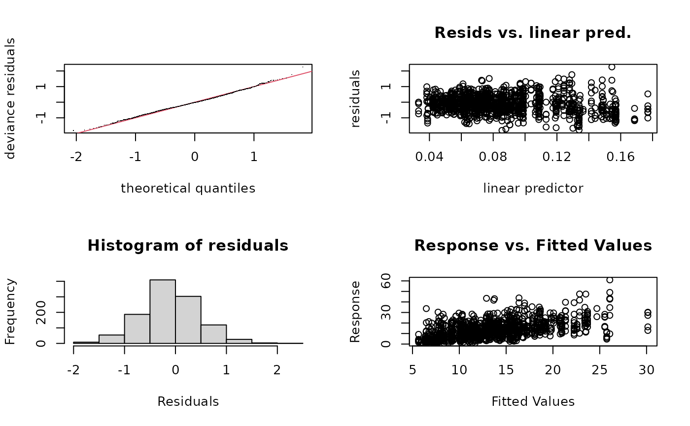

## 
## Method: GCV   Optimizer: outer newton
## full convergence after 8 iterations.
## Gradient range [6.886352e-11,6.377734e-07]
## (score 0.3332369 & scale 0.3350731).
## Hessian positive definite, eigenvalue range [7.71641e-06,0.0001997042].
## Model rank =  15 / 15 
## 
## Basis dimension (k) checking results. Low p-value (k-index<1) may
## indicate that k is too low, especially if edf is close to k'.
## 
##                              k'  edf k-index p-value    
## s(lunar.date):Speciesmono  3.00 2.79    0.72  <2e-16 ***
## s(lunar.date):Speciespsac5 3.00 2.99    0.72  <2e-16 ***
## s(month):Speciesmono       3.00 2.26    0.72  <2e-16 ***
## s(month):Speciespsac5      3.00 2.93    0.72  <2e-16 ***
## ---
## Signif. codes:  0 '***' 0.001 '**' 0.01 '*' 0.05 '.' 0.1 ' ' 1

And finally a summary of the best model using:

summary(best.model)

## 
## Family: Gamma 
## Link function: inverse 
## 
## Formula:
## GSI ~ s(lunar.date, by = Species, k = 5, bs = "cc") + s(month, 
##     by = Species, k = 5, bs = "cc") + Sex + Species
## 
## Parametric coefficients:
##               Estimate Std. Error t value Pr(>|t|)    
## (Intercept)   0.078944   0.002427  32.527  < 2e-16 ***
## Sexmale      -0.020572   0.002652  -7.757 1.98e-14 ***
## Speciespsac5  0.031402   0.002996  10.482  < 2e-16 ***
## ---
## Signif. codes:  0 '***' 0.001 '**' 0.01 '*' 0.05 '.' 0.1 ' ' 1
## 
## Approximate significance of smooth terms:
##                              edf Ref.df      F p-value    
## s(lunar.date):Speciesmono  2.787      3  3.702 0.00783 ** 
## s(lunar.date):Speciespsac5 2.988      3 42.745 < 2e-16 ***
## s(month):Speciesmono       2.263      3 10.552 < 2e-16 ***
## s(month):Speciespsac5      2.926      3 28.425 < 2e-16 ***
## ---
## Signif. codes:  0 '***' 0.001 '**' 0.01 '*' 0.05 '.' 0.1 ' ' 1
## 
## R-sq.(adj) =  0.296   Deviance explained = 28.4%
## GCV = 0.33324  Scale est. = 0.33507   n = 1110

Note all predictors are highly significant in this model, which we would typically expect given it was selected by AICc.

We can make a prettier plot to visualise the best model using some custom base R code.

model.dat=model.set$used.data
head(model.dat)

##         GSI Species    Sex year month.label month act.date       date
## 1  7.690040    mono female    3         Jul     7        8 2003-07-08
## 2  7.019802    mono female    3         Jul     7        8 2003-07-08
## 3 18.355220    mono female    3         Jul     7        8 2003-07-08
## 4  9.303880    mono female    3         Jul     7        8 2003-07-08
## 5 16.057208    mono female    3         Jul     7        8 2003-07-08
## 6  7.636143    mono female    3         Jul     7        8 2003-07-08
##   lunar.date   gwt    swt rep.id Sex.I.Species
## 1          9 18.26 237.45     28   female mono
## 2          9 35.45 505.00     30   female mono
## 3          9 50.04 272.62     37   female mono
## 4          9 27.84 299.23     41   female mono
## 5          9 50.41 313.94     44   female mono
## 6          9 42.88 561.54     46   female mono

str(model.dat)

## 'data.frame':    1110 obs. of  13 variables:
##  $ GSI          : num  7.69 7.02 18.36 9.3 16.06 ...
##  $ Species      : Factor w/ 2 levels "mono","psac5": 1 1 1 1 1 1 1 1 1 1 ...
##  $ Sex          : Factor w/ 2 levels "female","male": 1 1 1 1 1 1 1 2 1 2 ...
##  $ year         : Factor w/ 2 levels "3","4": 1 1 1 1 1 1 1 1 1 1 ...
##  $ month.label  : chr  "Jul" "Jul" "Jul" "Jul" ...
##  $ month        : int  7 7 7 7 7 7 7 7 7 7 ...
##  $ act.date     : int  8 8 8 8 8 8 8 8 8 8 ...
##  $ date         : chr  "2003-07-08" "2003-07-08" "2003-07-08" "2003-07-08" ...
##  $ lunar.date   : int  9 9 9 9 9 9 9 9 9 9 ...
##  $ gwt          : num  18.3 35.5 50 27.8 50.4 ...
##  $ swt          : num  237 505 273 299 314 ...
##  $ rep.id       : int  28 30 37 41 44 46 47 50 51 53 ...
##  $ Sex.I.Species: Factor w/ 4 levels "female mono",..: 1 1 1 1 1 1 1 3 1 3 ...

x.seq=seq(from=1,to=30,length=100)

best.mod.fact.vars=c("Sex","Species")
fact.grid=unique(model.dat[,best.mod.fact.vars])
sex.ltys=c(1,2)
sex.pchs=c(19,21)
sex.lvls=levels(model.dat$Sex)
spp.lvls=levels(model.dat$Species)
sex.cols=c("blue","red")

# create some symbology and colour schemes for plotting
model.dat$pchs=16
for(a in 1:length(sex.lvls)){
    model.dat$cols[which(model.dat$Sex==sex.lvls[a])]=sex.cols[a]}

y.lim=c(0,ceiling(max(model.dat$GSI)))
lunar.lim=range(model.dat$lunar.date)
lunar.seq=seq(from=1,to=30,length=100)
month.lim=range(model.dat$month)
month.seq=seq(from=1,to=30,length=100)

month.labels=c("Jan","Feb","Mar","Apr","May","Jun","Jul","Aug","Sep","Oct","Nov","Dec")

spp.labels=c("Monodonta labio", "Patelloida saccharina")

par(mfcol=c(2,2),mar=c(0,0.5,0.5,0.5),oma=c(5,4,0.5,2))
for(x in 1:length(spp.lvls)){
# lunar
spp=spp.lvls[x]
fact.grid.plot=fact.grid[grep(spp,fact.grid$Species),]
plot.dat=model.dat[grep(spp,model.dat$Species),]
plot(NA,ylim=y.lim,xlim=lunar.lim,ylab="",xlab="",main="",xpd=NA,yaxt="n",xaxt="n")
axis(side=2)
if(x==2){axis(side=1)}
for(r in 1:nrow(fact.grid.plot)){
 pred.vals=predict(best.model,newdata=data.frame(
                                      lunar.date=lunar.seq,
                                      month=mean(model.dat$month),
                                      Species=spp,
                                      Sex=fact.grid.plot[r,"Sex"]),
                                      type="response",se=T)
 lines(x.seq,pred.vals$fit,lwd=1.5,
       col=sex.cols[which(fact.grid.plot[r,"Sex"]==sex.lvls)])
 lines(x.seq,pred.vals$fit+1.96*pred.vals$se,lty=3,lwd=1.5,
       col=sex.cols[which(fact.grid.plot[r,"Sex"]==sex.lvls)])
 lines(x.seq,pred.vals$fit-1.96*pred.vals$se, lty=3,lwd=1.5,
       col=sex.cols[which(fact.grid.plot[r,"Sex"]==sex.lvls)])}
points(jitter(plot.dat$lunar.date),plot.dat$GSI,pch=16,col=plot.dat$cols)}
# month
for(x in 1:length(spp.lvls)){
spp=spp.lvls[x]
fact.grid.plot=fact.grid[grep(spp,fact.grid$Species),]
plot.dat=model.dat[grep(spp,model.dat$Species),]
plot(NA,ylim=y.lim,xlim=month.lim,ylab="",xlab="",main="",xpd=NA,yaxt="n",xaxt="n")
#if(x==1){axis(side=2)}
if(x==2){axis(side=1,at=c(2,4,6,8,10,12),labels=month.labels[c(2,4,6,8,10,12)])}
for(r in 1:nrow(fact.grid.plot)){
 pred.vals=predict(best.model,newdata=data.frame(
                                      lunar.date=mean(model.dat$lunar.date),
                                      month=month.seq,
                                      Species=spp,
                                      Sex=fact.grid.plot[r,"Sex"]),
                                      type="response",se=T)
 lines(x.seq,pred.vals$fit,lwd=1.5,
       col=sex.cols[which(fact.grid.plot[r,"Sex"]==sex.lvls)])
 lines(x.seq,pred.vals$fit+1.96*pred.vals$se,lty=3,lwd=1.5,
       col=sex.cols[which(fact.grid.plot[r,"Sex"]==sex.lvls)])
 lines(x.seq,pred.vals$fit-1.96*pred.vals$se, lty=3,lwd=1.5,
       col=sex.cols[which(fact.grid.plot[r,"Sex"]==sex.lvls)])}
points(jitter(plot.dat$month),plot.dat$GSI,pch=16,col=plot.dat$cols)}

mtext(side=1,text=c("Lunar date","Month of the year"),at=c(0.25,0.75),outer=T,line=2.5)
mtext(side=2,text="GSI",outer=T,line=2)
mtext(side=4,text=spp.labels,at=c(0.75,0.25),outer=T)
legend.dat=unique(model.dat[,c("Sex","cols")])
legend.dat=legend.dat[order(legend.dat$Sex),]

legend("bottom",legend=paste(legend.dat$Sex),bty="n",cex=1,
       inset=-0.275,ncol=2,lty=1,col=legend.dat$cols,pch=16,xpd=NA)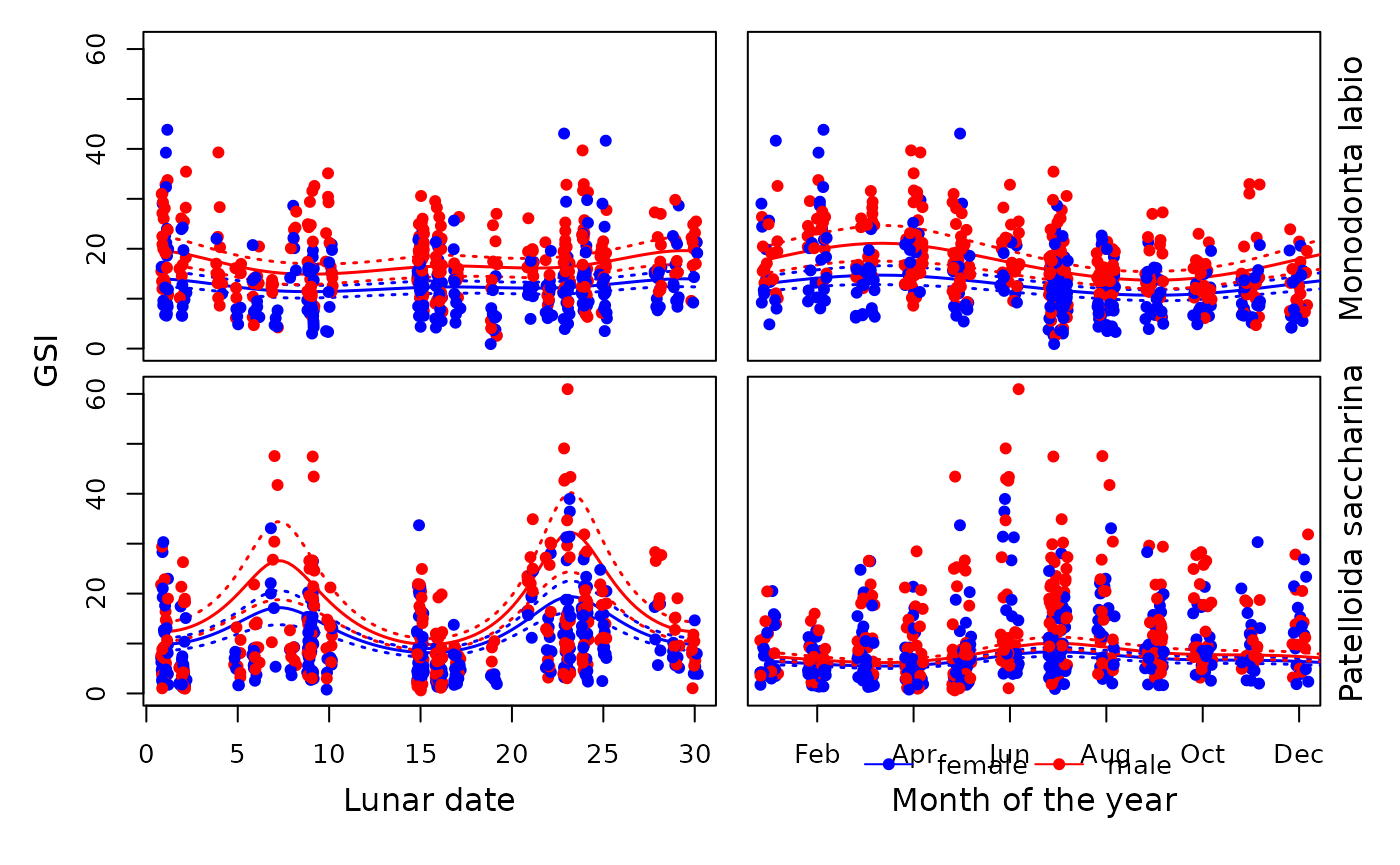

Results and discussion

The most strongly supported model included cyclic smooths of both lunar date and month interacting with species, combined with a main effect of sex. This model explained approximately 28% of the variance in GSI.

Strong semi‑lunar patterns were observed for Patelloida saccharina, with peaks occurring approximately twice per lunar cycle. In contrast, Monodonta labio exhibited weaker and phase‑shifted lunar responses. Seasonal patterns also differed between species, with peak reproductive output occurring at different times of the year.

Overall, this case study demonstrates the value of GAMs with cyclic splines and interaction structures for dissecting complex reproductive rhythms across multiple temporal scales.