Case Study 2 • FSSgam.docs

Overview

This case study reanalyses data from Langlois et al. (2005) to examine whether large reef-associated predators (rock lobster and snapper) structure adjacent soft‑sediment communities. The analysis demonstrates the use of full subsets GAMMs in the FSSgam package, accounting for nested random effects and zero‑inflated abundance data.

Background

In ecology, ‘haloes’ have been described in many contexts (Suchanek 1978; Fairweather 1988) and generally are thought to result from a predator or herbivore foraging given distances from a ‘shelter habitat’ out into a ‘food habitat’. Studies in temperate marine ecosystems have found ‘infaunal haloes’, areas of decreased density of soft-sediment fauna adjacent to reefs, at a variety of scales (0-30 m, (Davis et al. 1982); 0-70 m, (Posey and Ambrose 1994)). The model suggesting reef-associated predators are responsible for haloes is supported by studies of gut contents of fish on temperate reefs (Lindquist et al. 1994). However, convincing demonstrations of predators causing haloes of prey in these systems have been hampered due to limited replication of caging studies (Posey and Ambrose 1994) and the lack of large-scale manipulations (Thrush et al. 2000).

The most conspicuous predators associated with reefs in northeastern New Zealand are the sparid fish Pagrus auratus (snapper) and the rock lobster Jasus edwardsii. They are highly targeted by local fisheries and occur at higher densities inside no‑take marine reserves (NTR, Babcock et al. 1999). In this region the influence of predators on rocky reefs has been examined using the existing large-scale experimental framework provided by marine reserves (Babcock et al. 1999; Shears and Babcock 2002). Using this approach, Langlois et al. (2005) examined the potential role of large reef-associated predators in structuring adjacent soft-sediment communities, by contrasting the densities of predators and prey found inside versus outside three NTR.

Unlike a Before-After-Control-Impact (Underwood 1993) designed study, a potential problem with studies of established NTR is that evidence of a negative relationship between predator densities and densities of prey does not eliminate other potential models (Hurlbert 1984; Underwood et al. 2000). Results might be confounded by other factors that may structure the soft-sediment community (e.g. wave action, sediment grain-size distributions, organic matter, infaunal interactions). In the original study, Langlois et al. (2005) hypothesised that predation by large reef-associated predators would result in lower densities of large (> 4 mm) soft-sediment macrofauna inside reserves compared to outside reserves (Predator model). A further hypothesis was that predation would decrease with increasing distances from the reef, resulting in a ‘halo’ pattern in the community (Posey and Ambrose 1994), i.e., an increase in prey densities with increasing distances from the reef edge (Distance model).

In the original study, Langlois et al. (2005) investigated the influence of measured environmental variables (see the variable table in Methods, below) on the abundance composition of the assemblage inside and outside multiple NTR using multivariate multiple regression, which found no evidence that any of the measured environmental variables were confounding the comparison of the soft-sediment assemblages inside and outside the multiple NTR. To estimate effects on individual taxa inside and outside the NTR across the multiple random sites and multiple NTR locations, the original analysis used a mixed-model ANOVA, where P-values were obtained using permutations (Anderson and Braak 2003), to account for the great many zeros contained in the data. Any influence of the multiple environmental variables measured could not be accounted for in the original analysis of individual taxa due to the limited error families available in GLMM routines at that time. As a consequence it was impossible to tease apart the relative importance of NTR status and distance from the reef edge from variation in snapper or rock lobster density or the influence of measured environmental variables on the individual infaunal taxa. The revised analyses here based on a full subsets multiple regression approach allows the influence of environmental and predator density variables to be assessed independently, whilst accounting for the nesting of random sites inside and outside multiple random NTR and samples collected along a transect of fixed distance from the reef edge.

Methods

In 2002 New Zealand’s northeastern bioregion contained eight reserves, three of which were considered broadly comparable biotype replicates (Shears and Babcock 2003; Willis et al. 2003). This study was carried out between January and March of 2002, using these three locations as a random factor to explicitly test the generality of any potential differences in the effects of marine reserve status (as in Beck 1997). The Cape Rodney to Okakari Point (Leigh) Marine Reserve (36°16’S, 174°48’E) was gazetted in 1975, the Tawharanui Marine Park (36°22’S, 174°50’E) was declared a no-take area in 1981 and the Te Whanganui a Hei (Hahei) Marine Reserve (36°50’S, 175°49’E) was gazetted in 1993. At each location eight sites of similar wave exposure and reef/soft-sediment interfaces were chosen, four inside and four outside each marine reserve, with non-reserve sites interspersed both north and south of the reserve to mitigate the potential confounding influence of other environmental variables (such as recruitment or food supply).

Within each site, sampling was done at each of four distances from the reef edge: 2, 5, 15 and 30 m. These distance strata were comparable to previous studies of infaunal haloes (Posey and Ambrose 1994) and within the likely foraging ranges of snapper (Parsons et al. 2003) and rock lobster (Kelly et al. 1999). At each distance, six replicate samples were obtained using box quadrats measuring 0.5 m² (1 m x 0.5 m) x 13 cm deep (0.065 m³). Sediment was excavated by hand with a metal scoop and sieved in the field using a sieve with a 4 mm mesh. Other studies from different systems (Ambrose 1991; Lindquist et al. 1994; Posey and Ambrose 1994; Dahlgren et al. 1999) have focused on smaller infauna (> 0.5 mm) where the corresponding reef-associated predators were also smaller. In the present study, we focused on larger infauna (> 4 mm), corresponding to the larger reef-associated predators found within reserves (snapper are ~316 mm mean total length and rock lobster are ~109.9 mm mean carapace length inside reserves, (Babcock et al. 1999)). Organisms retained on the sieve were preserved in 5% formalin and later transferred to 70% ethanol, and identified to the lowest taxonomic resolution possible.

Physical environmental variables measured at each distance stratum at each site included replicate measurements of grain size by dry sieving, organic content by ignition at 550°C, and bed form measurements. Wave exposure was estimated using an index of potential fetch (Thomas 1986). Estimates of the density of snapper at the reef edge were obtained using baited underwater video (BUV, Willis and Babcock 2000). Estimates of the density of lobster at the reef edge were obtained by underwater visual census (UVC, MacDiarmid 1991). A list and brief description of the environmental variables measured and subsequently included in analyses are given below.

Environmental variables used as predictors in the full subsets analyses.
Variable	Description
Snapper	Density of legal-sized snapper (Pagrus auratus) estimated by BUV
Rock Lobster	Density of legal-sized rock lobster (Jasus edwardsii) estimated by UVC
Predatory Infauna	Infauna considered to be predators (Langlois et al. 2005)
Bioturbating Infauna	Infauna considered to be bioturbators (Langlois et al. 2005)
Grain size fractions	Percentage of grain sizes of ambient sediments (by weight), from 125 um up to 4 mm
Organics	Sediment organic matter (%)
Bed Stress	Estimated using bed form ripple measurements and depth
Exposure	Estimation of fetch (km)
Depth	Water depth (m)

Analysis

A generalised additive mixed model with full subsets analyses was used to determine if NTR status, distance from the reef edge, variation in snapper or rock lobster density or the influence of any measured environmental variables or interactions between these predictors best explained variance in abundance of the three most abundant and ubiquitous infaunal taxa. Abundance data were modelled using a tweedie distribution, implemented via a call to gam (mgcv, (Wood 2017)) with the random effect of site included using the bs='re' specification. Smoothers to the random factors of NTR location and nested sites (bs='re') were included in all models (and as part of the null model) via the null.terms argument of the full subsets gam function. Given the complexity of the null model, the total number of predictors was limited to only an additional three terms (max.predictors=3) and k was limited to 3. As the density of legal-sized lobster and snapper and NTR status were all relevant to the primary hypothesis, the most parsimonious models within 2 AIC units of the top model that contained any of these variables in addition to any habitat variables were considered as the most parsimonious. The R language for statistical computing (R Core Team 2017) was used for all data manipulation (dplyr, Wickham and Francois 2016; tidyr, Wickham 2017), analysis (mgcv, Wood 2011) and graphing (ggplot2, Wickham 2009; gridExtra, Auguie 2016).

** note ** This example was updated on the 11th Oct 2018 to demonstrate usage of the replacement functions generate_model_set and fit_model_set that have now superseded full.subsets.gam in package FSSgam Between them these functions carry out the same analysis, take the same arguments and return the same outputs as full.subsets.gam with the only difference being that the model set generation and model fitting procedures are separated into two steps. This was done to make the function easier to use, because the model set can be interrogated, along with the correlation matrix of the predictors before model fitting is even attempted.

It has since been updated with minimal changes on the 29th April 2026 to ensure reproducibility and to convert it to a .Rmd file for the vignette format for githubio.

It was updated again on the dev branch to call generate_model_set and fit_model_set, the snake_case names that generate.model.set and fit.model.set were themselves renamed to. The old dot-case names still work (they now just emit a deprecation warning and forward to the new names), but new code should call generate_model_set/fit_model_set directly.

Script information

Part 1-FSS modeling

This script is designed to work with long format data - where response variables are stacked one upon each other (see http://tidyr.tidyverse.org/)

There are two random factors, Site and NTR location We have used a Tweedie error distribution to account for the high occurence of zero values in the dataset. We have implemented the ramdom effects and Tweedie error distribution using the mgcv() package

Part 2 - custom plot of importance scores

Using ggplot2()

Part 3 - plots of the most parsimonious models

Here we use plots of the raw response variables and fitted relationships - to allow for the plotting of interactions between continous predictor variables and factors with levels again using ggplot2()

R packages

library(tidyr)
library(dplyr)
library(mgcv)
library(MuMIn)
library(car)
library(doBy)
library(gplots)
library(ggplot2)
library(RColorBrewer)
library(gamm4)
library(FSSgam)
library(gridExtra)
library(grid)

Part 1-FSS modeling

Data preparation

dat <-case_study2 %>%
  rename(response=Abundance)%>%
  #   Transform variables
  mutate(sqrt.X4mm=sqrt(X4mm))%>%
  mutate(sqrt.X2mm=sqrt(X2mm))%>%
  mutate(sqrt.X1mm=sqrt(X1mm))%>%
  mutate(sqrt.X500um=sqrt(X500um))%>%
  na.omit()%>%
  mutate(Location=factor(Location)) |> 
  mutate(Site=factor(Site)) |> 
  mutate(Status=factor(Status)) |> 
  glimpse()

## Rows: 285
## Columns: 25
## $ sediment    <dbl> -3.2625005, -3.4838280, -4.6855602, -3.2486536, -3.4328005…
## $ Location    <fct> Hahei, Hahei, Hahei, Hahei, Hahei, Hahei, Hahei, Hahei, Ha…
## $ Status      <fct> Fished, Fished, Fished, Fished, Fished, Fished, Fished, Fi…
## $ Site        <fct> Cooks Beach Inner, Cooks Beach Inner, Cooks Beach Inner, C…
## $ Distance    <int> 2, 5, 15, 30, 2, 5, 30, 2, 5, 15, 30, 2, 5, 15, 30, 2, 5, …
## $ depth       <int> 12, 12, 12, 12, 9, 9, 9, 10, 10, 12, 12, 10, 10, 11, 11, 1…
## $ X4mm        <dbl> 3.16462, 1.69129, 1.67228, 0.79670, 0.03768, 0.23887, 0.05…
## $ X2mm        <dbl> 1.41119, 1.62811, 1.01193, 0.77126, 0.25556, 0.57024, 0.41…
## $ X1mm        <dbl> 3.88962, 4.86726, 3.97180, 1.82919, 2.09768, 3.42348, 2.96…
## $ X500um      <dbl> 8.69694, 9.92831, 21.37884, 7.81927, 15.76419, 18.22572, 1…
## $ X250um      <dbl> 70.31984, 69.18594, 64.74207, 78.20548, 67.41767, 62.77750…
## $ X125um      <dbl> 6.19663, 5.70317, 2.75041, 5.26789, 7.21756, 7.48086, 2.31…
## $ X63um       <dbl> 6.25038, 6.92941, 4.42267, 5.27693, 7.08857, 7.17101, 3.47…
## $ fetch       <dbl> 2232582.5, 2232582.5, 2232582.5, 2232582.5, 1027166.9, 102…
## $ org         <dbl> 3.45785, 3.19104, 2.80046, 2.78881, 2.47510, 2.52552, 2.30…
## $ snapper     <dbl> 0.0, 0.0, 0.0, 0.0, 0.0, 0.0, 0.0, 0.0, 0.0, 0.0, 0.0, 0.0…
## $ lobster     <dbl> 0.0, 0.0, 0.0, 0.0, 0.2, 0.2, 0.2, 0.0, 0.0, 0.0, 0.0, 0.0…
## $ InPreds     <dbl> 0.0000000, 0.0000000, 0.0000000, 0.3333333, 0.0000000, 1.0…
## $ BioTurb     <dbl> 0.1666667, 0.1666667, 0.8333333, 0.3333333, 0.3333333, 0.1…
## $ Taxa        <chr> "BDS", "BDS", "BDS", "BDS", "BDS", "BDS", "BDS", "BDS", "B…
## $ response    <int> 0, 1, 0, 1, 6, 5, 1, 0, 0, 0, 0, 0, 0, 1, 3, 0, 4, 0, 2, 0…
## $ sqrt.X4mm   <dbl> 1.7789379, 1.3004961, 1.2931667, 0.8925805, 0.1941134, 0.4…
## $ sqrt.X2mm   <dbl> 1.1879352, 1.2759741, 1.0059473, 0.8782141, 0.5055294, 0.7…
## $ sqrt.X1mm   <dbl> 1.9722120, 2.2061868, 1.9929375, 1.3524755, 1.4483370, 1.8…
## $ sqrt.X500um <dbl> 2.9490575, 3.1509221, 4.6237258, 2.7962958, 3.9704143, 4.2…

Predictor selection

pred.vars=c("depth","X4mm","X2mm","X1mm","X500um","X250um","X125um","X63um",
            "fetch","org","snapper","lobster") 

factor.vars <- c("Status")

Predictor variables Removed at first pass included: broad.Sponges and broad.Octocoral.Black and broad.Consolidated , “InPreds”,“BioTurb” are too rare

Check for correalation of predictor variables- remove anything highly correlated (>0.95)—

round(cor(dat[,pred.vars]),2)

##         depth  X4mm  X2mm  X1mm X500um X250um X125um X63um fetch   org snapper
## depth    1.00  0.24  0.05 -0.01   0.02   0.10  -0.08  0.03  0.21  0.05   -0.16
## X4mm     0.24  1.00  0.52  0.21   0.03   0.13  -0.20  0.48  0.03  0.23   -0.11
## X2mm     0.05  0.52  1.00  0.91   0.58   0.10  -0.51  0.01  0.28  0.13    0.08
## X1mm    -0.01  0.21  0.91  1.00   0.80   0.09  -0.60 -0.17  0.38  0.06    0.14
## X500um   0.02  0.03  0.58  0.80   1.00   0.21  -0.74 -0.13  0.46  0.00    0.07
## X250um   0.10  0.13  0.10  0.09   0.21   1.00  -0.80  0.07  0.16  0.10   -0.22
## X125um  -0.08 -0.20 -0.51 -0.60  -0.74  -0.80   1.00 -0.05 -0.37 -0.09    0.10
## X63um    0.03  0.48  0.01 -0.17  -0.13   0.07  -0.05  1.00 -0.23  0.11   -0.11
## fetch    0.21  0.03  0.28  0.38   0.46   0.16  -0.37 -0.23  1.00  0.15    0.16
## org      0.05  0.23  0.13  0.06   0.00   0.10  -0.09  0.11  0.15  1.00    0.16
## snapper -0.16 -0.11  0.08  0.14   0.07  -0.22   0.10 -0.11  0.16  0.16    1.00
## lobster  0.09 -0.10  0.03  0.11   0.12  -0.24   0.10 -0.04  0.11  0.14    0.54
##         lobster
## depth      0.09
## X4mm      -0.10
## X2mm       0.03
## X1mm       0.11
## X500um     0.12
## X250um    -0.24
## X125um     0.10
## X63um     -0.04
## fetch      0.11
## org        0.14
## snapper    0.54
## lobster    1.00

Note that nothing is highly correlated

Plot of likely transformations - thanks to Anna Cresswell for this loop!

par(mfrow=c(3,2))
for (i in pred.vars) {
  x<-dat[ ,i]
  x = as.numeric(unlist(x))
  hist((x))#Looks best
  plot((x),main = paste(i))
  hist(sqrt(x))
  plot(sqrt(x))
  hist(log(x+1))
  plot(log(x+1))
}

Review of individual predictors - we have to make sure they have an even distribution.

If the data are squewed to low numbers try sqrt>log or if skewed to high numbers try ^2 of ^3 Decided that X4mm, X2mm, X1mm and X500um needed a sqrt transformation

Decided Depth, x63um, InPreds and BioTurb were not informative variables.

Re-set the predictors for modeling.

pred.vars=c("sqrt.X4mm","sqrt.X2mm","sqrt.X1mm","sqrt.X500um",
            "fetch","org","snapper","lobster")

Screening taxa

Check to make sure Response vector has not more than 80% zeros

unique.vars=unique(as.character(dat$Taxa))
unique.vars.use=character()
for(i in 1:length(unique.vars)){
  temp.dat=dat[which(dat$Taxa==unique.vars[i]),]
  if(length(which(temp.dat$response==0))/nrow(temp.dat)<0.8){
    unique.vars.use=c(unique.vars.use,unique.vars[i])}
}
unique.vars.use

## [1] "BDS" "BMS" "CPN"

“BDS” bivalve Dosina subrosea

“BMS” bivalve Myadora striata

“CPN” crustacean Pagrus novaezelandiae

Full subsets GAMM analysis

Extract Model fits and importance

names(out.all)=resp.vars
names(var.imp)=resp.vars
all.mod.fits=do.call("rbind",out.all)
all.var.imp=do.call("rbind",var.imp)

knitr::kable(
  all.mod.fits,
  digits = 3,
  caption = "Summary of all fitted FSSgam models"
)

Summary of all fitted FSSgam models
	modname	formula	AICc	BIC	r2.vals	r2.vals.unique	edf	delta.AICc	delta.BIC	wi.AICc	wi.BIC	sqrt.X4mm	fetch	org	lobster	Status	Distance	cumsum.wi
BDS.Distance+sqrt.X4mm	Distance+sqrt.X4mm	s(sqrt.X4mm, k = 3, bs = “cr”) + Distance + s(Location, Site, bs = “re”)	276.405	321.906	0.529	NA	23.24	0.000	0.000	0.677	0.721	1	0	0	0	0	1	0.677
BDS.Distance.t.Status+sqrt.X4mm+Status	Distance.t.Status+sqrt.X4mm+Status	s(sqrt.X4mm, k = 3, bs = “cr”) + Distance + Status + s(Location, Site, bs = “re”) + Distance:Status	277.884	323.807	0.517	NA	23.82	1.480	1.901	0.323	0.279	1	0	0	0	1	1	1.000
BMS.fetch.by.Status+sqrt.X4mm+Status	fetch.by.Status+sqrt.X4mm+Status	s(sqrt.X4mm, k = 3, bs = “cr”) + s(fetch, by = Status, k = 3, bs = “cr”) + Status + s(Location, Site, bs = “re”)	157.220	195.278	0.114	NA	15.70	0.000	0.000	0.630	0.909	1	1	0	0	1	0	0.630
BMS.fetch.by.Status+sqrt.X4mm.by.Status+Status	fetch.by.Status+sqrt.X4mm.by.Status+Status	s(fetch, by = Status, k = 3, bs = “cr”) + s(sqrt.X4mm, by = Status, k = 3, bs = “cr”) + Status + s(Location, Site, bs = “re”)	158.379	199.933	0.116	NA	17.70	1.159	4.655	0.353	0.089	1	1	0	0	1	0	0.983
CPN	lobster+org+sqrt.X4mm	s(lobster, k = 3, bs = “cr”) + s(org, k = 3, bs = “cr”) + s(sqrt.X4mm, k = 3, bs = “cr”) + s(Location, Site, bs = “re”)	399.262	446.531	0.481	NA	24.75	0.000	0.000	0.988	0.983	1	0	1	1	0	0	0.988

knitr::kable(
  all.var.imp,
  digits = 3,
  caption = "Variable importance scores across response variables"
)

Variable importance scores across response variables
	sqrt.X4mm	sqrt.X1mm	fetch	org	snapper	lobster	Status	Distance
BDS	1.000	0.000	0	0.000	0.000	0.000	0.323	1.000
BMS	0.984	0.000	1	0.000	0.017	0.000	0.983	0.013
CPN	0.988	0.013	0	1.001	0.000	0.996	0.005	0.000

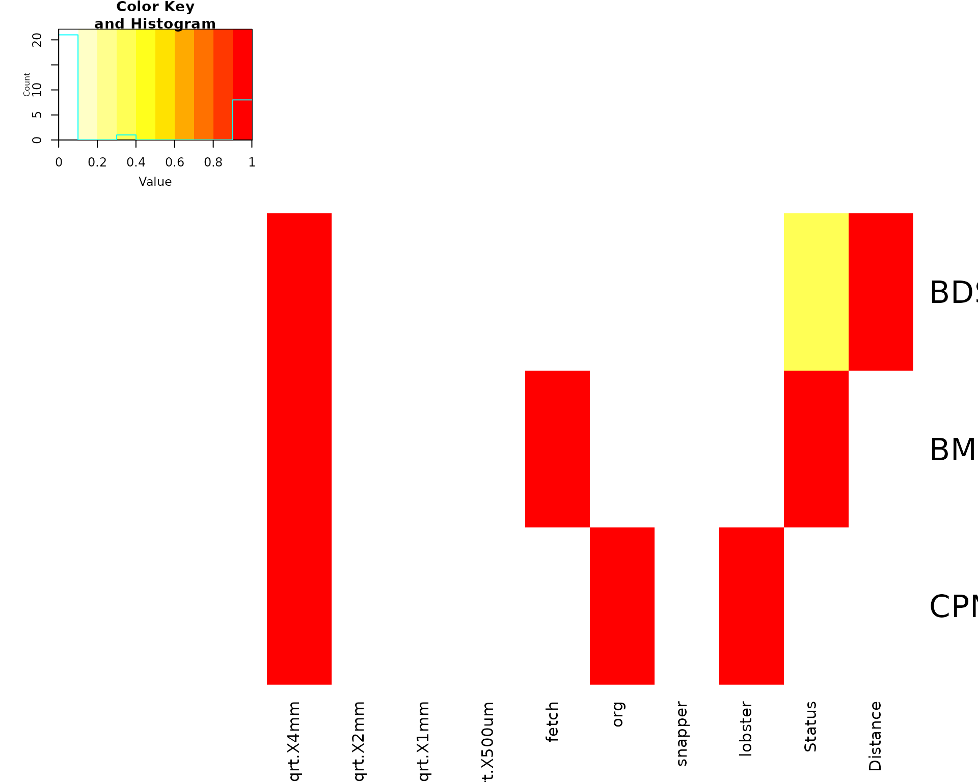
Variable importance

heatmap.2(
  all.var.imp,
  dendrogram = "none",
  col = colorRampPalette(c("white", "yellow", "red"))(10),
  trace = "none",
  key = TRUE,
  notecol = "black",
  sepcolor = "black",
  margins = c(6, 4),
  Rowv = FALSE,
  Colv = FALSE
)

Part 2 - custom plot of importance scores

dat.taxa <- all.var.imp |>
  as.data.frame() |>
  tibble::rownames_to_column("resp.var") |>
  pivot_longer(
    cols = -resp.var,
    names_to = "predictor",
    values_to = "importance"
  ) |>
  glimpse()

## Rows: 30
## Columns: 3
## $ resp.var   <chr> "BDS", "BDS", "BDS", "BDS", "BDS", "BDS", "BDS", "BDS", "BD…
## $ predictor  <chr> "sqrt.X4mm", "sqrt.X2mm", "sqrt.X1mm", "sqrt.X500um", "fetc…
## $ importance <dbl> 1.000, 0.000, 0.000, 0.000, 0.000, 0.000, 0.000, 0.000, 0.3…

gg.importance.scores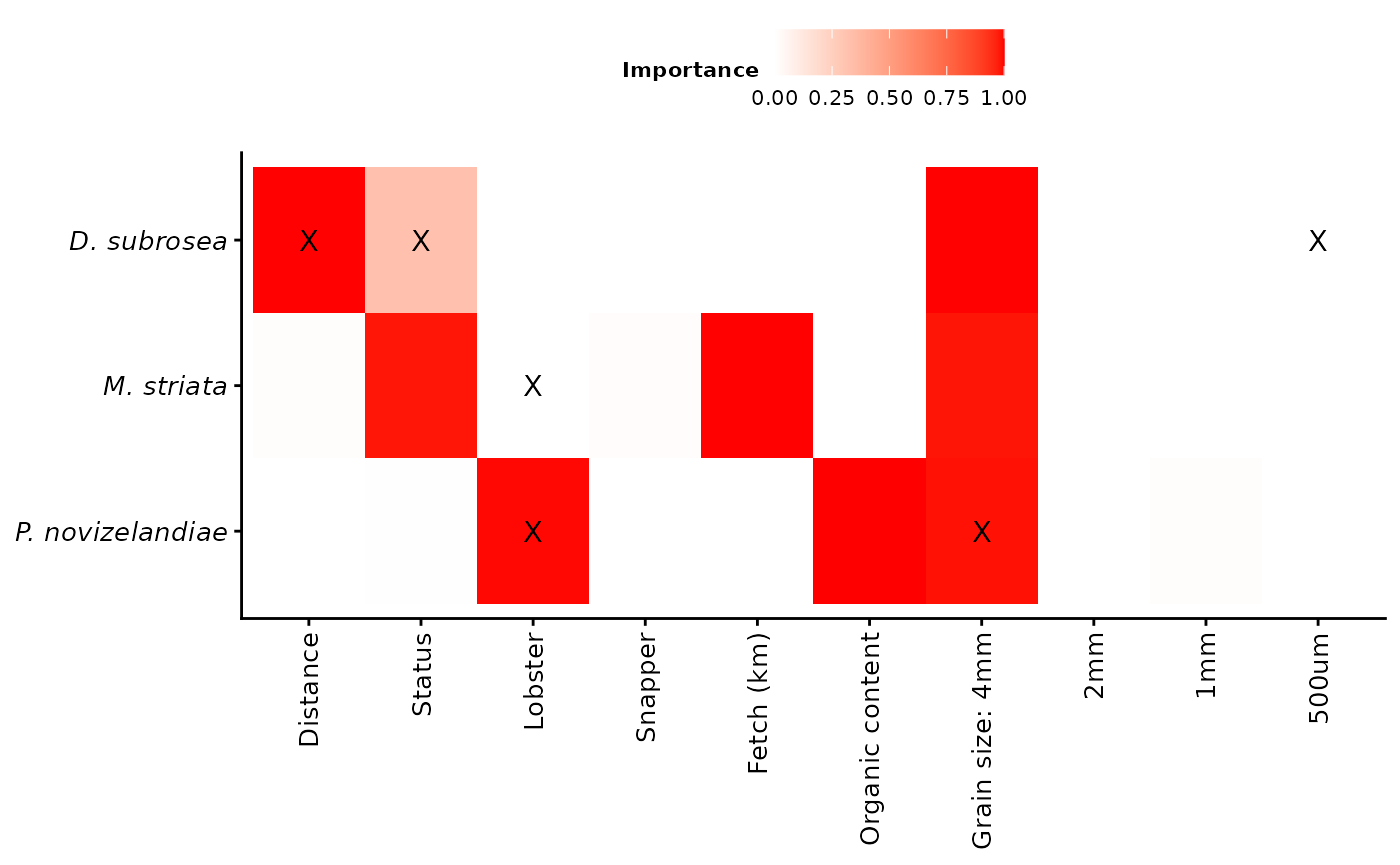

Part 3 - plots of the most parsimonious models

Make an suitable theme

Theme1 <- theme(
  panel.grid.major = element_blank(),
  panel.grid.minor = element_blank(),
  legend.background = element_blank(),
  legend.key = element_blank(),
  legend.text = element_text(size = 15),
  legend.title = element_blank(),
  legend.position = c(0.2, 0.8),
  text = element_text(size = 15),
  strip.text.y = element_text(size = 15, angle = 0),
  axis.title.x = element_text(vjust = 0.3, size = 15),
  axis.title.y = element_text(vjust = 0.6, angle = 90, size = 15),
  axis.text.x = element_text(size = 15),
  axis.text.y = element_text(size = 15),
  axis.line.x = element_line(colour = "black", linewidth = 0.5, linetype = "solid"),
  axis.line.y = element_line(colour = "black", linewidth = 0.5, linetype = "solid"),
  strip.background = element_blank()
)
name<-"clams"

Manually make the most parsimonious GAM models for each taxa

MODEL Bivalve.Dosina.subrosea 500um + Distance x Status

dat.bds<-dat%>%filter(Taxa=="BDS")
gamm=gam(response~s(sqrt.X500um,k=3,bs='cr')+s(Distance,k=1,bs='cr', by=Status)+ s(Location,Site,bs="re")+ Status, family=tw(),data=dat.bds)

Predict - status from MODEL Bivalve.Dosina.subrosea—-

mod<-gamm
testdata <- expand.grid(Distance=mean(mod$model$Distance),
                        sqrt.X500um=mean(mod$model$sqrt.X500um),
                        Location=(mod$model$Location),
                        Site=(mod$model$Site),
                        Status = c("Fished","No-take"))%>%
  distinct()%>%
  glimpse()

## Rows: 144
## Columns: 5
## $ Distance    <dbl> 12.97895, 12.97895, 12.97895, 12.97895, 12.97895, 12.97895…
## $ sqrt.X500um <dbl> 2.855525, 2.855525, 2.855525, 2.855525, 2.855525, 2.855525…
## $ Location    <fct> Hahei, Leigh, Tawharanui, Hahei, Leigh, Tawharanui, Hahei,…
## $ Site        <fct> Cooks Beach Inner, Cooks Beach Inner, Cooks Beach Inner, C…
## $ Status      <fct> Fished, Fished, Fished, Fished, Fished, Fished, Fished, Fi…

fits <- predict.gam(mod, newdata=testdata, type='response', se.fit=T)

predicts.bds.status = testdata%>%data.frame(fits)%>%
  group_by(Status)%>% #only change here
  summarise(response=mean(fit),se.fit=mean(se.fit))%>%
  ungroup()

predicts.bds.status %>%
  glimpse()

## Rows: 2
## Columns: 3
## $ Status   <fct> Fished, No-take
## $ response <dbl> 2.8646047, 0.7276123
## $ se.fit   <dbl> 2.390011, 0.619802

predict - Distance.x.status from MODEL Bivalve.Dosina.subrosea—-

mod<-gamm
testdata <- expand.grid(Distance=seq(min(dat$Distance),max(dat$Distance),length.out = 20),
                        sqrt.X500um=mean(mod$model$sqrt.X500um),
                        Location=(mod$model$Location),
                        Site=(mod$model$Site),
                        Status = c("Fished","No-take"))%>%
  distinct()%>%
  glimpse()

## Rows: 2,880
## Columns: 5
## $ Distance    <dbl> 2.000000, 3.473684, 4.947368, 6.421053, 7.894737, 9.368421…
## $ sqrt.X500um <dbl> 2.855525, 2.855525, 2.855525, 2.855525, 2.855525, 2.855525…
## $ Location    <fct> Hahei, Hahei, Hahei, Hahei, Hahei, Hahei, Hahei, Hahei, Ha…
## $ Site        <fct> Cooks Beach Inner, Cooks Beach Inner, Cooks Beach Inner, C…
## $ Status      <fct> Fished, Fished, Fished, Fished, Fished, Fished, Fished, Fi…

fits <- predict.gam(mod, newdata=testdata, type='response', se.fit=T)

predicts.bds.Distance.x.status = testdata%>%data.frame(fits)%>%
  group_by(Distance,Status)%>% 
  summarise(response=mean(fit),se.fit=mean(se.fit))%>%
  ungroup()
predicts.bds.Distance.x.status |> 
  glimpse()

## Rows: 40
## Columns: 4
## $ Distance <dbl> 2.000000, 2.000000, 3.473684, 3.473684, 4.947368, 4.947368, 6…
## $ Status   <fct> Fished, No-take, Fished, No-take, Fished, No-take, Fished, No…
## $ response <dbl> 2.0505723, 0.4356395, 2.1446873, 0.4666912, 2.2431218, 0.4999…
## $ se.fit   <dbl> 1.7306685, 0.3823930, 1.8058795, 0.4073529, 1.8848049, 0.4341…

Predict 500um from MODEL Bivalve.Dosina.subrosea—-

mod<-gamm
testdata <- expand.grid(sqrt.X500um=seq(min(dat$sqrt.X500um),max(dat$sqrt.X500um),length.out = 20),
                        Distance=mean(mod$model$Distance),
                        Location=(mod$model$Location),
                        Site=(mod$model$Site),
                        Status = c("Fished","No-take"))%>%
  distinct()%>%
  glimpse()

## Rows: 2,880
## Columns: 5
## $ sqrt.X500um <dbl> 0.4630875, 0.7521858, 1.0412841, 1.3303825, 1.6194808, 1.9…
## $ Distance    <dbl> 12.97895, 12.97895, 12.97895, 12.97895, 12.97895, 12.97895…
## $ Location    <fct> Hahei, Hahei, Hahei, Hahei, Hahei, Hahei, Hahei, Hahei, Ha…
## $ Site        <fct> Cooks Beach Inner, Cooks Beach Inner, Cooks Beach Inner, C…
## $ Status      <fct> Fished, Fished, Fished, Fished, Fished, Fished, Fished, Fi…

fits <- predict.gam(mod, newdata=testdata, type='response', se.fit=T)

predicts.bds.500um = testdata%>%data.frame(fits)%>%
  group_by(sqrt.X500um)%>% 
  summarise(response=mean(fit),se.fit=mean(se.fit))%>%
  ungroup()
predicts.bds.500um %>%
  glimpse()

## Rows: 20
## Columns: 3
## $ sqrt.X500um <dbl> 0.4630875, 0.7521858, 1.0412841, 1.3303825, 1.6194808, 1.9…
## $ response    <dbl> 4.6448757, 4.1410544, 3.6918819, 3.2914306, 2.9344158, 2.6…
## $ se.fit      <dbl> 4.0647102, 3.5813495, 3.1606276, 2.7942131, 2.4748134, 2.1…

MODEL Bivalve.Myadora.striata Lobster

dat.bms<-dat%>%filter(Taxa=="BMS")
head(dat.bms,2)

##    sediment Location Status              Site Distance depth    X4mm    X2mm
## 1 -3.262500    Hahei Fished Cooks Beach Inner        2    12 3.16462 1.41119
## 2 -3.483828    Hahei Fished Cooks Beach Inner        5    12 1.69129 1.62811
##      X1mm  X500um   X250um  X125um   X63um   fetch     org snapper lobster
## 1 3.88962 8.69694 70.31984 6.19663 6.25038 2232582 3.45785       0       0
## 2 4.86726 9.92831 69.18594 5.70317 6.92941 2232582 3.19104       0       0
##   InPreds   BioTurb Taxa response sqrt.X4mm sqrt.X2mm sqrt.X1mm sqrt.X500um
## 1       0 0.1666667  BMS        6  1.778938  1.187935  1.972212    2.949057
## 2       0 0.1666667  BMS        4  1.300496  1.275974  2.206187    3.150922

gamm=gam(response~s(lobster,k=3,bs='cr')+ s(Location,Site,bs="re"), family=tw(),data=dat.bms)

# predict - lobster from model for Bivalve.Myadora.striata ----
mod<-gamm
testdata <- expand.grid(lobster=seq(min(dat$lobster),max(dat$lobster),length.out = 20),
                        Location=(mod$model$Location),
                        Site=(mod$model$Site),
                        Status = c("Fished","No-take"))%>%
  distinct()%>%
  glimpse()

## Rows: 2,880
## Columns: 4
## $ lobster  <dbl> 0.0000000, 0.3421053, 0.6842105, 1.0263158, 1.3684211, 1.7105…
## $ Location <fct> Hahei, Hahei, Hahei, Hahei, Hahei, Hahei, Hahei, Hahei, Hahei…
## $ Site     <fct> Cooks Beach Inner, Cooks Beach Inner, Cooks Beach Inner, Cook…
## $ Status   <fct> Fished, Fished, Fished, Fished, Fished, Fished, Fished, Fishe…

fits <- predict.gam(mod, newdata=testdata, type='response', se.fit=T)
predicts.bms.lobster = testdata%>%data.frame(fits)%>%
  group_by(lobster)%>% 
  summarise(response=mean(fit),se.fit=mean(se.fit))%>%
  ungroup()

predicts.bms.lobster %>%
  glimpse()

## Rows: 20
## Columns: 3
## $ lobster  <dbl> 0.0000000, 0.3421053, 0.6842105, 1.0263158, 1.3684211, 1.7105…
## $ response <dbl> 1.93534254, 1.56507086, 1.26563993, 1.02349643, 0.82768005, 0…
## $ se.fit   <dbl> 1.73352921, 1.38496562, 1.11267638, 0.89887748, 0.72994634, 0…

MODEL Decapod.P.novazelandiae 4mm + Lobster

dat.cpn<-dat%>%filter(Taxa=="CPN")
head(dat.cpn,2)

##    sediment Location Status              Site Distance depth    X4mm    X2mm
## 1 -3.262500    Hahei Fished Cooks Beach Inner        2    12 3.16462 1.41119
## 2 -3.483828    Hahei Fished Cooks Beach Inner        5    12 1.69129 1.62811
##      X1mm  X500um   X250um  X125um   X63um   fetch     org snapper lobster
## 1 3.88962 8.69694 70.31984 6.19663 6.25038 2232582 3.45785       0       0
## 2 4.86726 9.92831 69.18594 5.70317 6.92941 2232582 3.19104       0       0
##   InPreds   BioTurb Taxa response sqrt.X4mm sqrt.X2mm sqrt.X1mm sqrt.X500um
## 1       0 0.1666667  CPN        3  1.778938  1.187935  1.972212    2.949057
## 2       0 0.1666667  CPN       11  1.300496  1.275974  2.206187    3.150922

gamm=gam(response~s(sqrt.X4mm,k=3,bs='cr')+s(lobster,k=3,bs='cr')+ s(Location,Site,bs="re"), family=tw(),data=dat.cpn)

Predict - sqrt.X4mm from model for Decapod.P.novazelandiae —-

mod<-gamm
testdata <- expand.grid(sqrt.X4mm=seq(min(dat$sqrt.X4mm),max(dat$sqrt.X4mm),length.out = 20),
                        lobster=mean(mod$model$lobster),
                        Location=(mod$model$Location),
                        Site=(mod$model$Site),
                        Status = c("Fished","No-take"))%>%
  distinct()%>%
  glimpse()

## Rows: 2,880
## Columns: 5
## $ sqrt.X4mm <dbl> 0.00000000, 0.09362831, 0.18725662, 0.28088493, 0.37451324, …
## $ lobster   <dbl> 1.909474, 1.909474, 1.909474, 1.909474, 1.909474, 1.909474, …
## $ Location  <fct> Hahei, Hahei, Hahei, Hahei, Hahei, Hahei, Hahei, Hahei, Hahe…
## $ Site      <fct> Cooks Beach Inner, Cooks Beach Inner, Cooks Beach Inner, Coo…
## $ Status    <fct> Fished, Fished, Fished, Fished, Fished, Fished, Fished, Fish…

fits <- predict.gam(mod, newdata=testdata, type='response', se.fit=T)
predicts.cpn.4mm = testdata%>%data.frame(fits)%>%
  group_by(sqrt.X4mm)%>% #only change here
  summarise(response=mean(fit),se.fit=mean(se.fit))%>%
  ungroup()
predicts.cpn.4mm %>%
  glimpse()

## Rows: 20
## Columns: 3
## $ sqrt.X4mm <dbl> 0.00000000, 0.09362831, 0.18725662, 0.28088493, 0.37451324, …
## $ response  <dbl> 4.822420, 4.499149, 4.197548, 3.916164, 3.653641, 3.408715, …
## $ se.fit    <dbl> 3.235051, 2.979428, 2.751207, 2.547690, 2.366325, 2.204703, …

Predict - lobster from model for Decapod.P.novazelandiae —-

mod<-gamm
testdata <- expand.grid(lobster=seq(min(dat$lobster),max(dat$lobster),length.out = 20),
                        sqrt.X4mm=mean(mod$model$sqrt.X4mm),
                        Location=(mod$model$Location),
                        Site=(mod$model$Site),
                        Status = c("Fished","No-take"))%>%
  distinct()%>%
  glimpse()

## Rows: 2,880
## Columns: 5
## $ lobster   <dbl> 0.0000000, 0.3421053, 0.6842105, 1.0263158, 1.3684211, 1.710…
## $ sqrt.X4mm <dbl> 0.4572685, 0.4572685, 0.4572685, 0.4572685, 0.4572685, 0.457…
## $ Location  <fct> Hahei, Hahei, Hahei, Hahei, Hahei, Hahei, Hahei, Hahei, Hahe…
## $ Site      <fct> Cooks Beach Inner, Cooks Beach Inner, Cooks Beach Inner, Coo…
## $ Status    <fct> Fished, Fished, Fished, Fished, Fished, Fished, Fished, Fish…

fits <- predict.gam(mod, newdata=testdata, type='response', se.fit=T)
predicts.cpn.lobster = testdata%>%data.frame(fits)%>%
  group_by(lobster)%>% 
  summarise(response=mean(fit),se.fit=mean(se.fit))%>%
  ungroup()
predicts.cpn.lobster %>%
  glimpse()

## Rows: 20
## Columns: 3
## $ lobster  <dbl> 0.0000000, 0.3421053, 0.6842105, 1.0263158, 1.3684211, 1.7105…
## $ response <dbl> 4.560408, 4.334946, 4.120627, 3.916900, 3.723238, 3.539142, 3…
## $ se.fit   <dbl> 3.038395, 2.857564, 2.693471, 2.544742, 2.410040, 2.288081, 2…

PLOTS for Bivalve.Dosina.subrosea 500um + Distance x Status

ggmod.bds.status<- ggplot(aes(x=Status,y=response,fill=Status,colour=Status), data=predicts.bds.status) +
  ylab(" ")+
  xlab('Status')+
  scale_fill_manual(labels = c("Fished", "No-take"),values=c("red", "black"))+
  scale_colour_manual(labels = c("Fished", "No-take"),values=c("red", "black"))+
  scale_x_discrete(limits = rev(levels(predicts.bds.status$Status)))+
  geom_bar(stat = "identity")+
  geom_errorbar(aes(ymin = response-se.fit,ymax = response+se.fit),width = 0.5) +
  theme_classic()+
  Theme1+
  annotate("text", x = -Inf, y=Inf, label = "(a)",vjust = 1, hjust = -.1,size=5)+
  annotate("text", x = -Inf, y=Inf, label = "   Dosinia subrosea",vjust = 1, hjust = -.1,size=5,fontface="italic")
ggmod.bds.status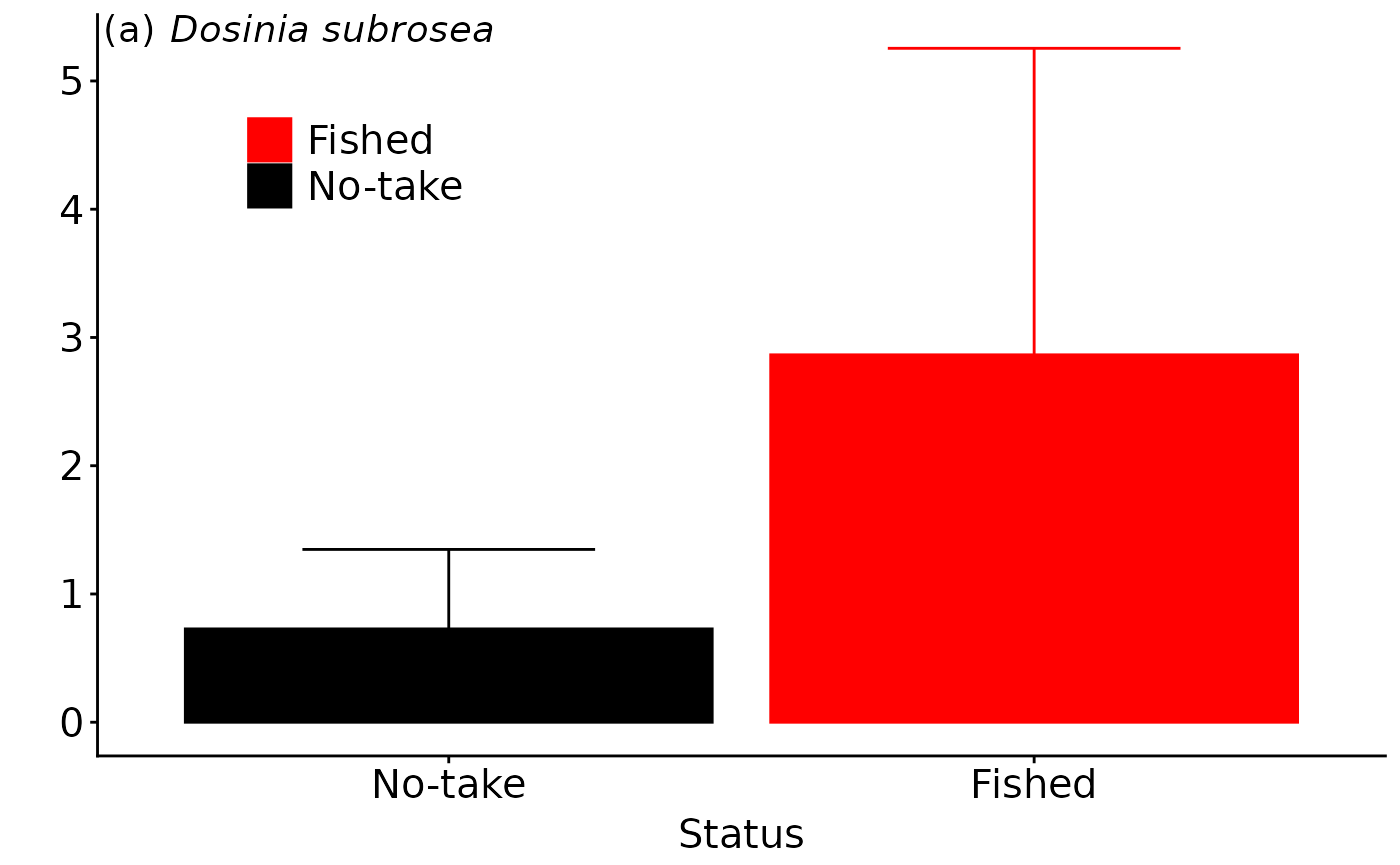

ggmod.bds.Distance.x.status<- ggplot(aes(x=Distance,y=response,colour=Status), data=dat.bds) +
  ylab(" ")+
  xlab('Distance (m)')+
  scale_color_manual(labels = c("Fished", "No-take"),values=c("red", "black"))+
  geom_jitter(width = 0.25,height = 0,alpha=0.75, size=2,show.legend=FALSE)+
  # geom_point(alpha=0.75, size=2)+
  geom_line(data=predicts.bds.Distance.x.status,show.legend=FALSE)+
  geom_line(data=predicts.bds.Distance.x.status,aes(y=response - se.fit),linetype="dashed",show.legend=FALSE)+
  geom_line(data=predicts.bds.Distance.x.status,aes(y=response + se.fit),linetype="dashed",show.legend=FALSE)+
  theme_classic()+
  Theme1+
  annotate("text", x = -Inf, y=Inf, label = "(b)",vjust = 1, hjust = -.1,size=5)
ggmod.bds.Distance.x.status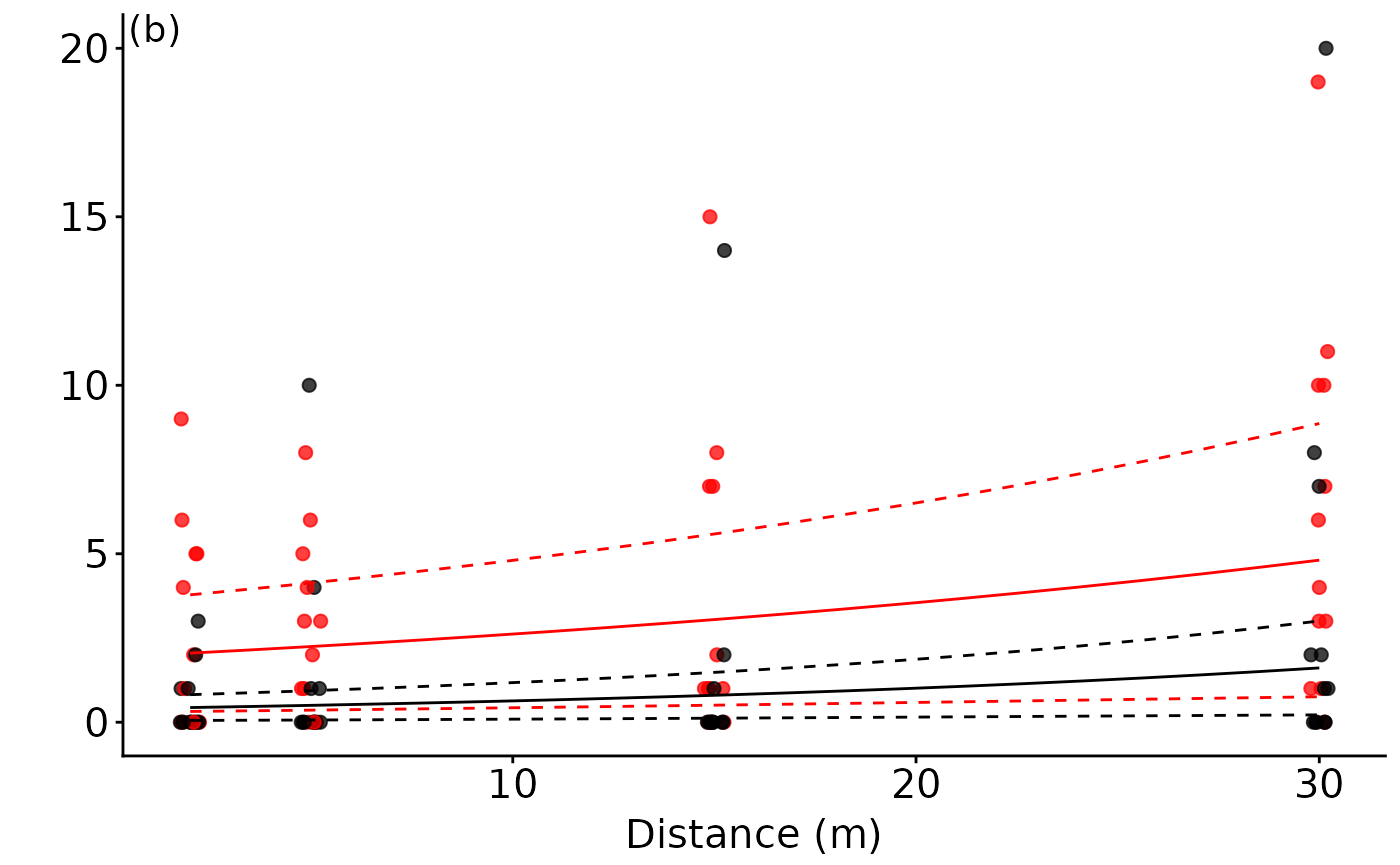

ggmod.bds.500um<- ggplot() +
  ylab(" ")+
  xlab('Grain size: 500 um (sqrt)')+
  scale_color_manual(labels = c("Fished", "No-take"),values=c("red", "black"))+
  geom_point(data=dat.bds,aes(x=sqrt.X500um,y=response,colour=Status),  alpha=0.75, size=2,show.legend=FALSE)+
  geom_line(data=predicts.bds.500um,aes(x=sqrt.X500um,y=response),alpha=0.5)+
  geom_line(data=predicts.bds.500um,aes(x=sqrt.X500um,y=response - se.fit),linetype="dashed",alpha=0.5)+
  geom_line(data=predicts.bds.500um,aes(x=sqrt.X500um,y=response + se.fit),linetype="dashed",alpha=0.5)+
  theme_classic()+
  Theme1+
  annotate("text", x = -Inf, y=Inf, label = "(c)",vjust = 1, hjust = -.1,size=5)
ggmod.bds.500um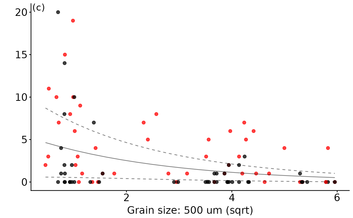

PLOTS Bivalve M.striata lobster

ggmod.bms.lobster<- ggplot() +
  ylab("Abundance")+
  xlab(bquote('Density of legal lobster (no./25' *m^-2*')'))+
  scale_color_manual(labels = c("Fished", "SZ"),values=c("red", "black"))+
  geom_point(data=dat.bms,aes(x=lobster,y=response,colour=Status),  alpha=0.75, size=2,show.legend=FALSE)+
  geom_line(data=predicts.bms.lobster,aes(x=lobster,y=response),alpha=0.5)+
  geom_line(data=predicts.bms.lobster,aes(x=lobster,y=response - se.fit),linetype="dashed",alpha=0.5)+
  geom_line(data=predicts.bms.lobster,aes(x=lobster,y=response + se.fit),linetype="dashed",alpha=0.5)+
  theme_classic()+
  Theme1+
  annotate("text", x = -Inf, y=Inf, label = "(d)",vjust = 1, hjust = -.1,size=5)+
  annotate("text", x = -Inf, y=Inf, label = "   Myadora striata",vjust = 1, hjust = -.1,size=5,fontface="italic")+
  geom_blank(data=dat.bms,aes(x=lobster,y=response*1.05))#to nudge data off annotations
ggmod.bms.lobster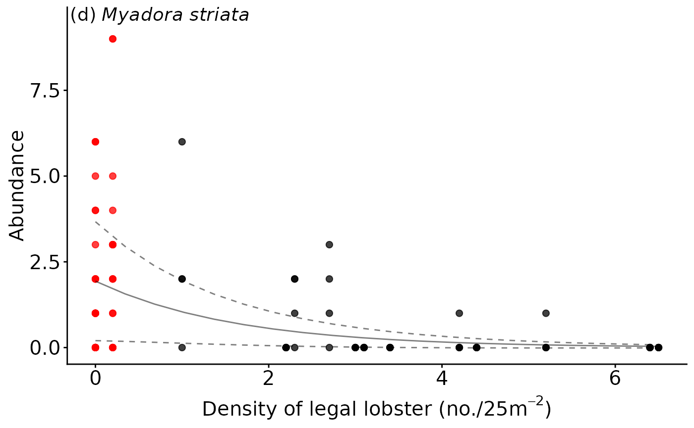

PLOTS Decapod.P.novazelandiae 4mm + lobster

ggmod.cpn.lobster<- ggplot() +
  ylab(" ")+
  xlab(bquote('Density of legal lobster (no./25' *m^-2*')'))+
  scale_color_manual(labels = c("Fished", "SZ"),values=c("red", "black"))+
  geom_point(data=dat.cpn,aes(x=lobster,y=response,colour=Status),  alpha=0.75, size=2,show.legend=FALSE)+
  geom_line(data=predicts.cpn.lobster,aes(x=lobster,y=response),alpha=0.5)+
  geom_line(data=predicts.cpn.lobster,aes(x=lobster,y=response - se.fit),linetype="dashed",alpha=0.5)+
  geom_line(data=predicts.cpn.lobster,aes(x=lobster,y=response + se.fit),linetype="dashed",alpha=0.5)+
  theme_classic()+
  Theme1+
  annotate("text", x = -Inf, y=Inf, label = "(e)",vjust = 1, hjust = -.1,size=5)+
  annotate("text", x = -Inf, y=Inf, label = "  Pagurus novizelandiae",vjust = 1, hjust = -.1,size=5,fontface="italic")+
  geom_blank(data=dat.cpn,aes(x=lobster,y=response*1.05))#to nudge data off annotations
ggmod.cpn.lobster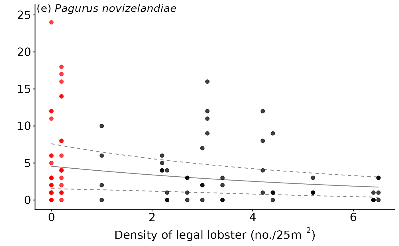

ggmod.cpn.4mm<- ggplot() +
  ylab(" ")+
  xlab('Grain size: 4 mm (sqrt)')+
  scale_color_manual(labels = c("Fished", "No-take"),values=c("red", "black"))+
  geom_point(data=dat.cpn,aes(x=sqrt.X4mm,y=response,colour=Status),  alpha=0.75, size=2,show.legend=FALSE)+
  geom_line(data=predicts.cpn.4mm,aes(x=sqrt.X4mm,y=response),alpha=0.5)+
  geom_line(data=predicts.cpn.4mm,aes(x=sqrt.X4mm,y=response - se.fit),linetype="dashed",alpha=0.5)+
  geom_line(data=predicts.cpn.4mm,aes(x=sqrt.X4mm,y=response + se.fit),linetype="dashed",alpha=0.5)+
  theme_classic()+
  Theme1+
  annotate("text", x = -Inf, y=Inf, label = "(f)",vjust = 1, hjust = -.1,size=5)+
  annotate("text", x = -Inf, y=Inf, label = " ",vjust = 1, hjust = -.1,size=5,fontface="italic")
ggmod.cpn.4mm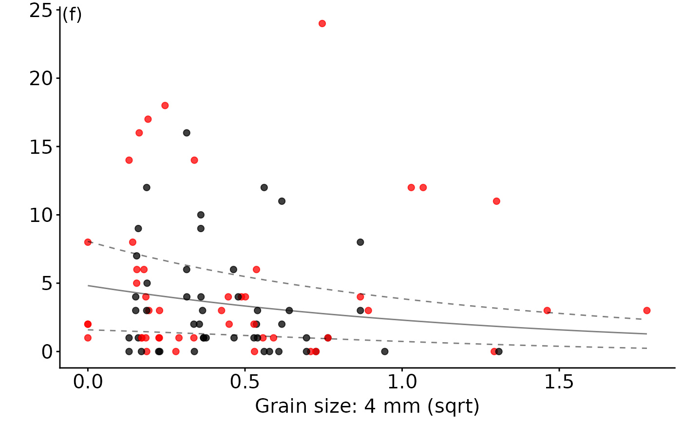

Combined.plot using grid() and gridExtra()

To see what they will look like use grid.arrange() - make sure Plot window is large enough! - or will error!

blank <- grid.rect(gp=gpar(col="white"))

grid.arrange(ggmod.bds.status,ggmod.bds.Distance.x.status,ggmod.bds.500um,
             ggmod.bms.lobster,blank,blank,
             ggmod.cpn.lobster,ggmod.cpn.4mm,blank,nrow=3,ncol=3)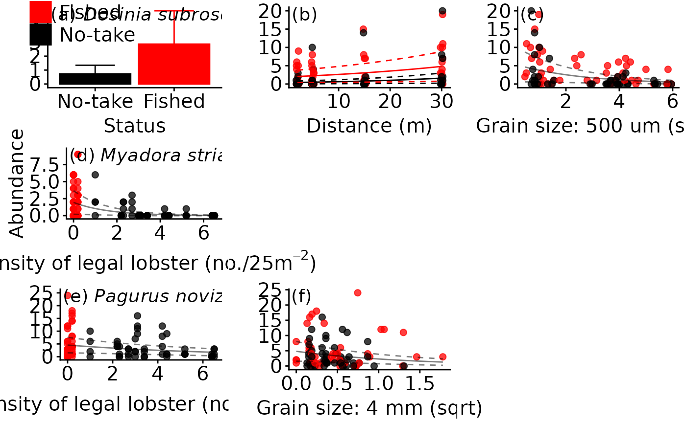

Use arrangeGrob ONLY - as we can pass this to ggsave! Note use of raw ggplot’s

combine.plot<-arrangeGrob(ggmod.bds.status,ggmod.bds.Distance.x.status,ggmod.bds.500um,
                          ggmod.bms.lobster,blank,blank,
                          ggmod.cpn.lobster,ggmod.cpn.4mm,blank,nrow=3,ncol=3)



combine.plot

## TableGrob (3 x 3) "arrange": 9 grobs
##   z     cells    name                grob
## 1 1 (1-1,1-1) arrange      gtable[layout]
## 2 2 (1-1,2-2) arrange      gtable[layout]
## 3 3 (1-1,3-3) arrange      gtable[layout]
## 4 4 (2-2,1-1) arrange      gtable[layout]
## 5 5 (2-2,2-2) arrange rect[GRID.rect.299]
## 6 6 (2-2,3-3) arrange rect[GRID.rect.299]
## 7 7 (3-3,1-1) arrange      gtable[layout]
## 8 8 (3-3,2-2) arrange      gtable[layout]
## 9 9 (3-3,3-3) arrange rect[GRID.rect.299]

Results and discussion

The most parsimonious model for the bivalve Dosinia subrosea included the interaction of distance from reef with NTR status and the 500 um sediment grain size fraction, which (along with random site effects) explained 52% of its distribution (see the model summary table above). While fetch occurred in the second top model, importance scores indicated that it was relatively unimportant compared to distance and NTR status (see the variable importance heatmap above). The abundance of D. subrosea was negatively correlated with increasing proportion of the 500 um sediment grain size fraction and positively correlated with increasing distance from the reef edge (see the plots above). Subsequent manipulative studies have found that D. subrosea are readily preyed upon by the large-bodied rock lobster in the field (Langlois, Anderson, Babcock, et al. 2006) and laboratory (Langlois, Anderson, Brock, et al. 2006), supporting the results of this analysis.

NTR status, distance and organic content were found to be important across all possible models explaining the abundance of Myadora striata, and had strong model support according to AICc. However a simpler model of decreasing abundance of M. striata with increasing density of legal-sized rock lobster was the most parsimonious model within 2 AICc, and had relatively high model support based on BIC. A direct relationship with the density of legal-sized rock lobster is consistent with the observation that greater than legal-size rock lobster can readily prey upon bivalves (Langlois, Anderson, Brock, et al. 2006).

There was a high level of model uncertainty in the full subsets analysis of the ubiquitous hermit crab Pagurus novizelandiae, with very low model weights and low, relatively evenly distributed variable importance scores. This is consistent with the original study that found no effect of NTR status on the abundance of Pagurus novizelandiae. The best model included the 4 mm sediment grain size fraction and the density of legal-sized rock lobster, explaining 48% of the distribution of P. novizelandiae. The abundance of P. novizelandiae was negatively correlated with increasing proportion of the 4 mm sediment grain size fraction and negatively correlated with the density of rock lobster on the reef edge. The direct relationship between the density of legal-sized rock lobster and the hermit crab P. novizelandiae is consistent with feeding studies of rock lobster, which indicated that they can exhibit a strong preference for decapod prey (Dumas et al. 2013).

Overall the general results of the revised analysis are comparable to those from the original study. However, by allowing environmental information to be included in the new analysis, whilst accounting for the nesting and random allocation of sites and NTR locations, a more informed comparison of the abundance of ubiquitous infaunal taxa has been made possible. In particular, it is useful that instead of relying on a simple comparison of NTR status to test hypotheses regarding predation of infauna, the role of the large carnivorous species protected within the NTR (e.g. rock lobster) can be more clearly indicated once it is included as a predictor variable in the models.

References

Ambrose, W. G. 1991. “Are Infaunal Predators Important in Structuring Marine Soft-Bottom Communities?” American Zoologist 31: 849–60.

Anderson, M. J., and C. J. F. ter Braak. 2003. “Permutation Tests for Multi-Factorial Analysis of Variance.” Journal of Statistical Computation and Simulation 73: 85–113.

Auguie, B. 2016. gridExtra: Miscellaneous Functions for ’Grid’ Graphics.

Babcock, R. C., S. Kelly, N. T. Shears, J. W. Walker, and T. J. Willis. 1999. “Changes in Community Structure in Temperate Marine Reserves.” Marine Ecology Progress Series 189: 125–34.

Beck, M. W. 1997. “Inference and Generality in Ecology - Current Problems and an Experimental Solution.” Oikos 78: 265–73.

Dahlgren, C. P., M. H. Posey, and A. W. Hulbert. 1999. “The Effects of Bioturbation on the Infaunal Community Adjacent to an Offshore Hardbottom Reef.” Bulletin of Marine Science 64: 21–34.

Davis, N., G. R. Vanblaricom, and P. K. Dayton. 1982. “Man-Made Structures on Marine Sediments: Effects on Adjacent Benthic Communities.” Marine Biology 70: 295–304.

Dumas, J.-P., T. J. Langlois, K. R. Clarke, and K. I. Waddington. 2013. “Strong Preference for Decapod Prey by the Western Rock Lobster Panulirus Cygnus.” Journal of Experimental Marine Biology and Ecology 439: 25–34.

Fairweather, P. G. 1988. “Predation Creates Haloes of Bare Space Among Prey on Rocky Seashores in New South Wales.” Journal of Experimental Marine Biology and Ecology 114: 261–73.

Hurlbert, S. H. 1984. “Pseudoreplication and the Design of Ecological Field Experiments.” Ecological Monographs 54: 187–212.

Kelly, S., A. B. MacDiarmid, and R. C. Babcock. 1999. “Characteristics of Spiny Lobster, Jasus Edwardsii, Aggregations in Exposed Reef and Sandy Areas.” Marine and Freshwater Research 50: 409–16.

Langlois, T. J., M. J. Anderson, and R. C. Babcock. 2005. “Reef-Associated Predators Influence Adjacent Soft-Sediment Communities.” Ecology 86: 1508–19.

Langlois, T. J., M. J. Anderson, R. C. Babcock, and S. Kato. 2006. “Marine Reserves Demonstrate Trophic Interactions Across Habitats.” Oecologia 147: 134–40.

Langlois, T. J., M. J. Anderson, M. Brock, and G. Murman. 2006. “Importance of Rock Lobster Size-Structure for Trophic Interactions: Choice of Soft-Sediment Bivalve Prey.” Marine Biology 149: 447–54.

Lindquist, D. G., L. B. Cahoon, I. E. Clavijo, et al. 1994. “Reef Fish Stomach Contents and Prey Abundance on Reef and Sand Substrata Associated with Adjacent Artificial and Natural Reefs in Onslow Bay, North Carolina.” Bulletin of Marine Science 55: 1994.

MacDiarmid, A. B. 1991. “Seasonal Changes in Depth Distribution Sex Ratio and Size Frequency of Spiny Lobster (Jasus Edwardsii) on a Coastal Reef in Northern New Zealand.” Marine Ecology Progress Series 70: 129–41.

Parsons, D. M., R. C. Babcock, R. K. S. Hankin, et al. 2003. “Snapper Pagrus Auratus (Sparidae) Home Range Dynamics: Acoustic Tagging Studies in a Marine Reserve.” Marine Ecology Progress Series 262: 253–65.

Posey, M. H., and W. G. Ambrose. 1994. “Effects of Proximity to an Offshore Hard-Bottom Reef on Infaunal Abundances.” Marine Biology 118: 745–53.

R Core Team. 2017. R: A Language and Environment for Statistical Computing. R Foundation for Statistical Computing.

Shears, N. T., and R. C. Babcock. 2002. “Marine Reserves Demonstrate Top-down Control of Community Structure on Temperate Reefs.” Oecologia 132: 131–42.

Shears, N. T., and R. C. Babcock. 2003. Quantitative Classification of New Zealand Rocky Coastal Community Types. Department of Conservation.

Suchanek, T. H. 1978. “The Ecology of Mytilus Edulis in Exposed Rocky Inter Tidal Communities.” Journal of Experimental Marine Biology and Ecology 31: 105–20.

Thomas, M. L. H. 1986. “A Physically Derived Exposure Index for Marine Shorelines.” Ophelia 25: 1–13.

Thrush, S. F., J. E. Hewitt, V. J. Cummings, M. O. Green, G. A. Funnell, and M. R. Wilkinson. 2000. “The Generality of Field Experiments: Interactions Between Local and Broad-Scale Processes.” Ecology 81: 399–415.

Underwood, A. J. 1993. “The Mechanics of Spatially Replicated Sampling Programmes to Detect Environmental Impacts in a Variable World.” Austral Ecology 18: 99–116.

Underwood, A. J., M. G. Chapman, and S. D. Connell. 2000. “Observations in Ecology: You Can’t Make Progress on Processes Without Understanding the Patterns.” Journal of Experimental Marine Biology and Ecology 250: 97–115.

Wickham, H. 2009. Ggplot2: Elegant Graphics for Data Analysis. Springer-Verlag.

Wickham, H. 2017. Tidyr: Easily Tidy Data with ’Spread()’ and ’Gather()’ Functions.

Wickham, H., and R. Francois. 2016. Dplyr: A Grammar of Data Manipulation.

Willis, T. J., and R. C. Babcock. 2000. “A Baited Underwater Video System for the Determination of Relative Density of Carnivorous Reef Fish.” Marine & Freshwater Research 51: 755–63.

Willis, T. J., R. B. Millar, and R. C. Babcock. 2003. “Protection of Exploited Fish in Temperate Regions: High Density and Biomass of Snapper Pagrus Auratus (Sparidae) in Northern New Zealand Marine Reserves.” The Journal of Applied Ecology 40: 214–27.

Wood, S. N. 2011. “Fast Stable Restricted Maximum Likelihood and Marginal Likelihood Estimation of Semiparametric Generalized Linear Models.” Journal of the Royal Statistical Society. Series B, Statistical Methodology 73: 3–36.

Wood, S. N. 2017. Generalized Additive Models: An Introduction with r. 2nd ed. CRC Press.