Overview
This case study examines how management zoning and habitat structure
influence abundance and biomass across multiple reef fish functional
groups. It uses full subsets generalised additive mixed models (GAMMs)
implemented in the FSSgam package to identify the most
important predictors across multiple response variables.
Background
Coral reef fish are highly diverse assemblages that provide important ecosystem services for millions of people (Pratchett et al. 2014). These services are however threatened by overfishing (Newton et al. 2007; MacNeil et al. 2015) and a loss of habitat, in particular corals (Wilson et al. 2006) and the structure they provide (Rogers et al. 2014). No-take reserves (NTR) promote higher abundance and biomass of fish (Russ 2002; McClanahan et al. 2009) and conserve ecosystem function (Graham et al. 2011). It is clear that NTR cannot prevent large scale disturbances, such as heat stress that cause extensive coral loss and decline in fish (Jones et al. 2004; Graham et al. 2008), however a reduction in local pressures in NTR may facilitate greater resilience of coral reefs (Hughes et al. 2010).
By examining patch reefs of differing habitat quality inside and outside of NTR within the Ningaloo marine park, Wilson et al. (2012) explored how habitat degradation and fishing influenced the abundance and biomass of fish from different functional groups. Explanatory variables in the original analyses were summarised using the scores from the two axes of a principal components analysis (PCA), making it impossible to tease apart the relative importance of variables that were correlated along the axis. The revised analyses here based on a full subsets multiple regression approach allows the influence of habitat variables to be assessed independently.
Methods
Benthic and fish communities on patch reefs within fished (n=35) and NTR (n=33) of the Ningaloo lagoon were surveyed to investigate the influence of habitat and fishing on coral reef fish. On each patch the seascape level of reef structure (complexity) was assessed using a six point scale, where 0 represents no vertical relief and 5 represents highly complex reefs with small overhangs and caves (Polunin and Roberts 1993). Finer scale physical reef structure (rugosity) was measured as the linear distance covered by a 3m length of chain fitted to the reef contour (Risk 1972). Benthic cover was quantified along a 5m line intercept transect using the categories: high complex corals such as Branching morphologies (HC), low complexity corals such as massive and encrusting morphologies (LC), and macroalgae (Macro).
Abundance and size of adult fish was estimated by a diver using a point count method. Large mobile fish were initially counted from the perimeter of the patch, after which the entire patch was surveyed for smaller site attached species. Fish were placed into broad functional groups based on their diets and biomass calculated from length weight relationships (Froese and Pauly 2011).
Data analysis
A generalised additive model with full subsets analyses was used to determine if fishing, habitat or interactions between these variables best explained variance in abundance and biomass of functional fish groups.
Data preparation
In the original analysis PCA was used to summarise habitat information and scores from principal components 1 and 2 were included in the full subsets analysis. Principal component 1 was positively correlated with complexity and rugosity, but negatively correlated with percent macroalgal cover, while principal component 2 was positively correlated with HC, but negatively correlated with LC. In the revised analysis scores from both principal components (Score1 and Score2) were again included as explanatory variables, along with percent cover estimates from line intercept transects (HC, LC, Macro), complexity and rugosity measures. Zone (fished or NTR) was included as an assessment of fishing pressure. The motivation for including the original PCA scores in the revised analysis was that this should provide a means of comparing if the raw habitat predictors have a stronger relationship with the fish abundance and biomass variables than the PCA aggregate.
data("case_study1")Some transformations were applied to ensure the predictors were relatively evenly distribution without their range. This is important to obtain stable results from FSSgam.
Outlier handling
FFSgam can also be very sensitive to outliers. In this case these were a small number of very large schools of fish, that would be unlikely to be closely linked to the habitat variables in any case.
case_study1$Piscivore.abundance[case_study1$Piscivore.abundance > 150] <- NA
case_study1$Piscivore.biomass[case_study1$Piscivore.biomass > 40000] <- NA
case_study1$Invertivore.biomass[case_study1$Invertivore.biomass > 40000] <- NA
Predictor specification
The categorical predictors and continuous predictors are passed to FSSgam via two separate vectors:
cat.preds <- "ZONE"
null.vars <- c("depth", "site", "SQRTSA")
cont.preds <- c(
"complexity", "sqrt.rug", "sqrtLC", "sqrtHC",
"sqrtMacro", "SCORE1", "SCORE2"
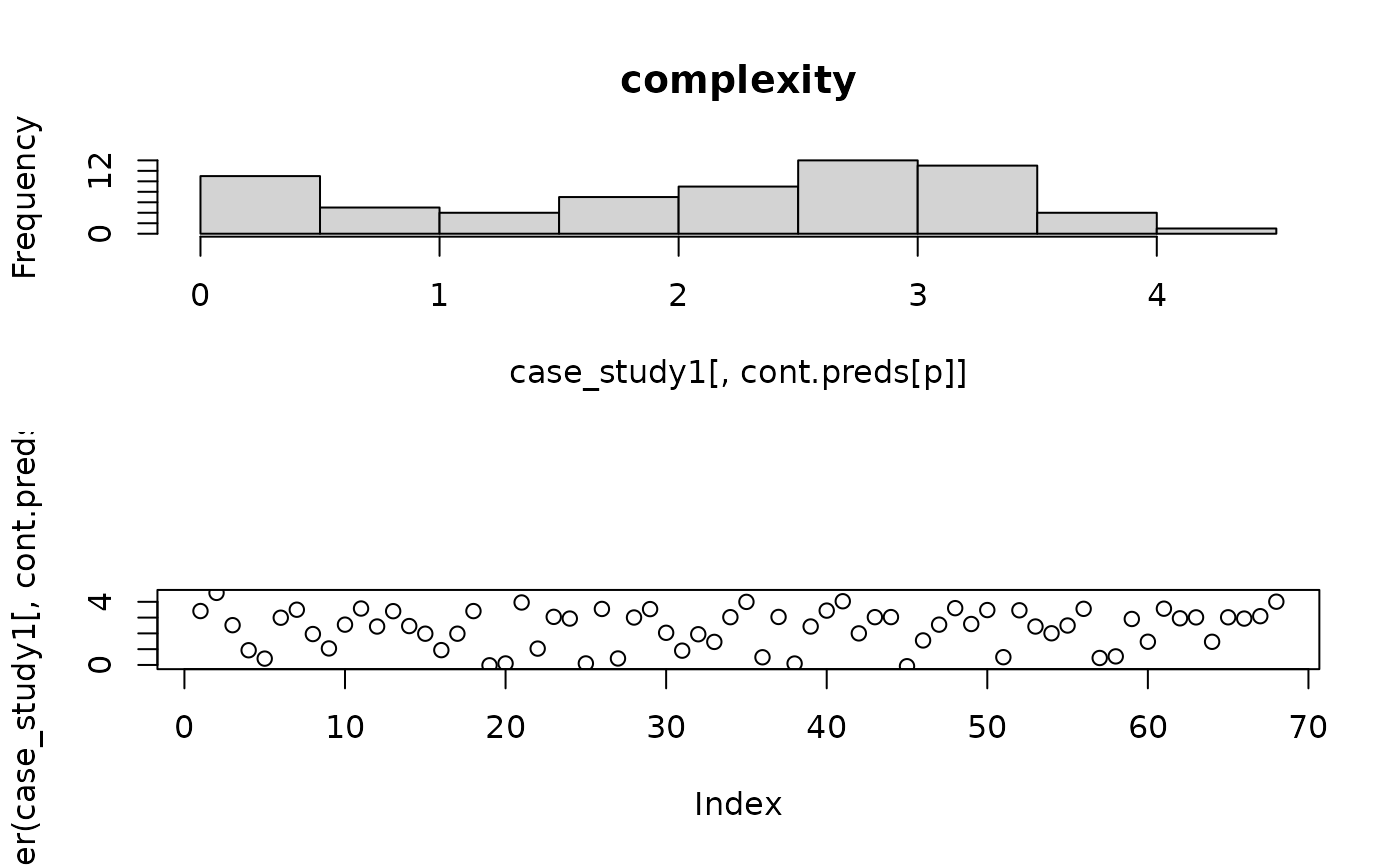
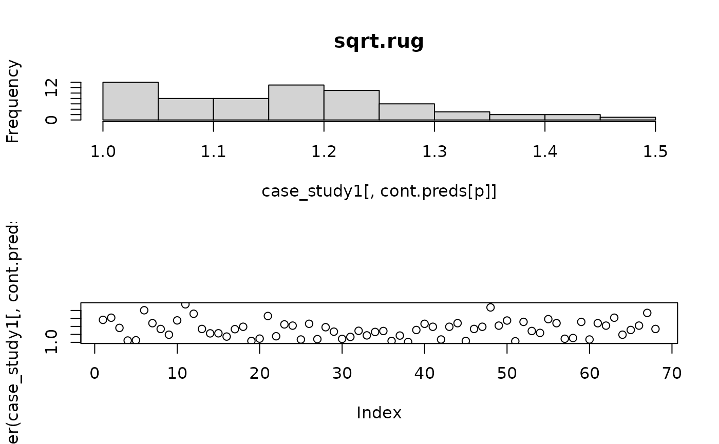
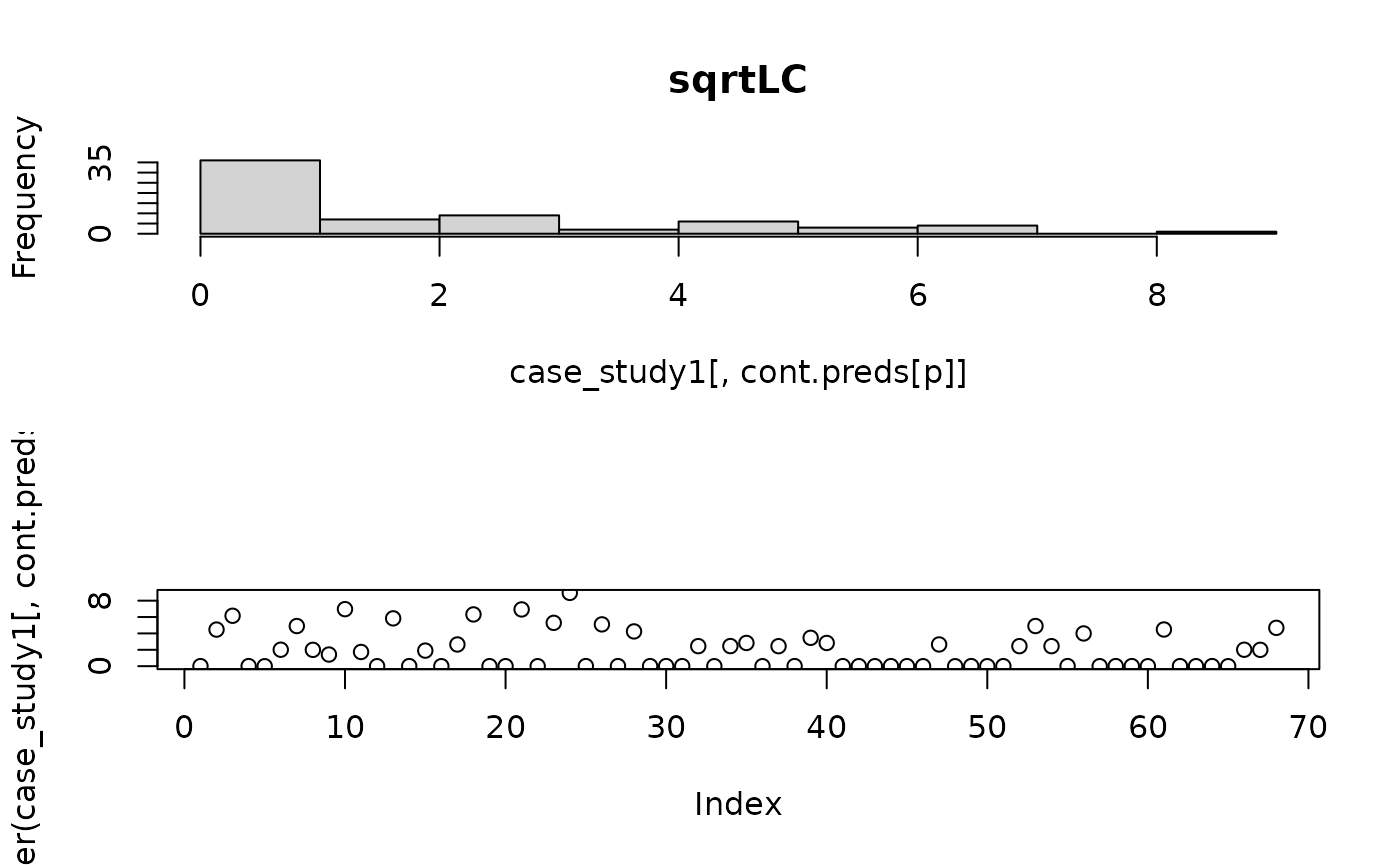
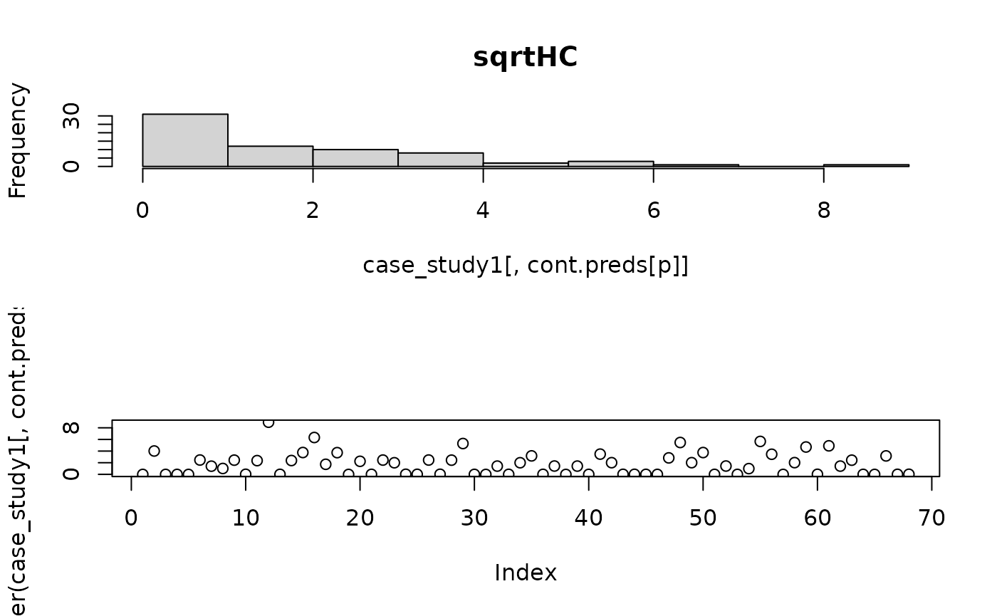
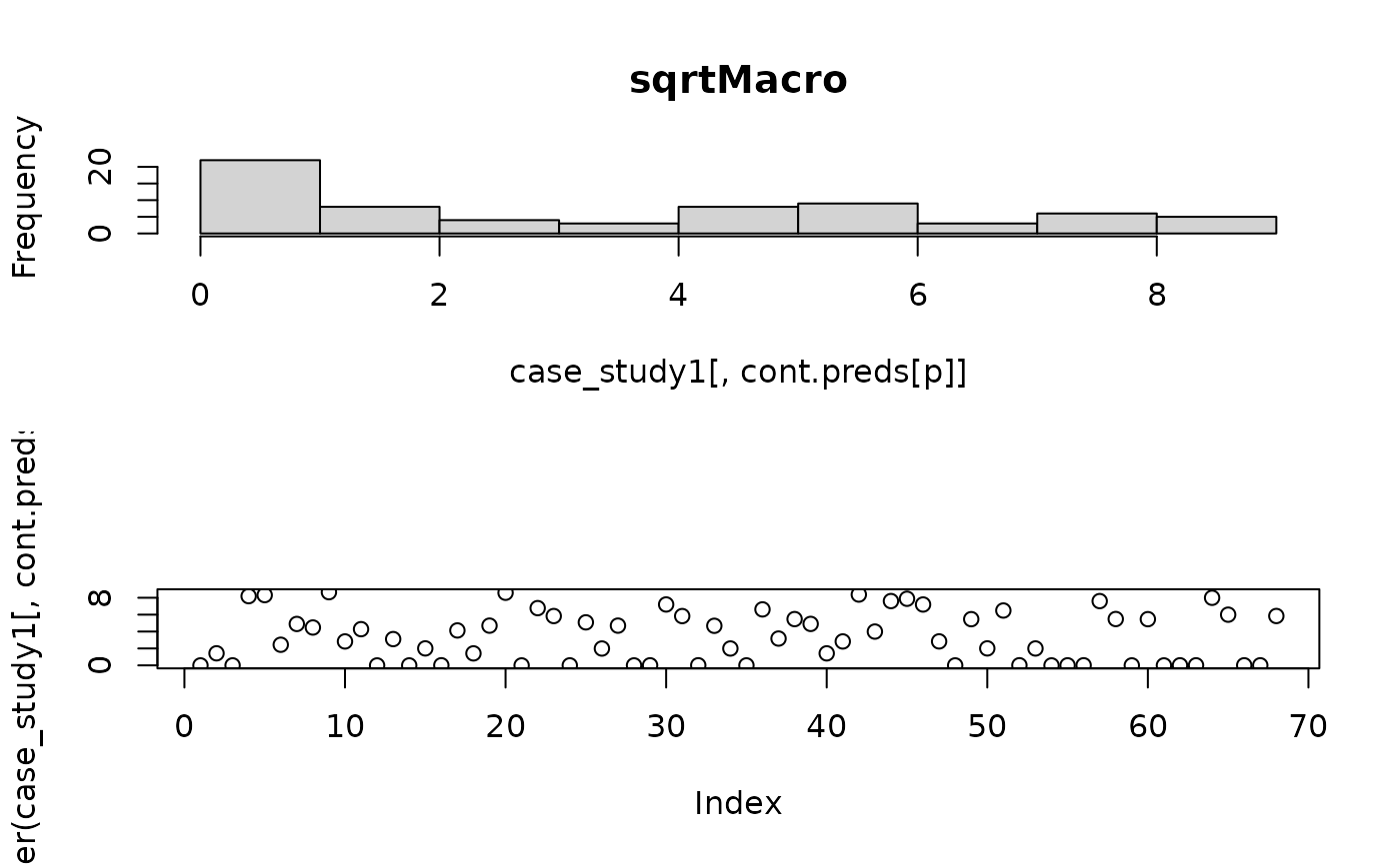
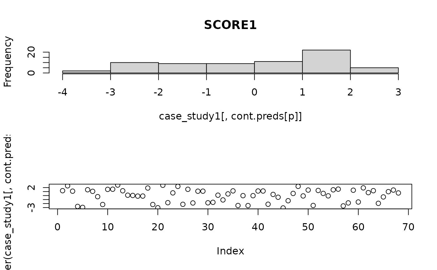
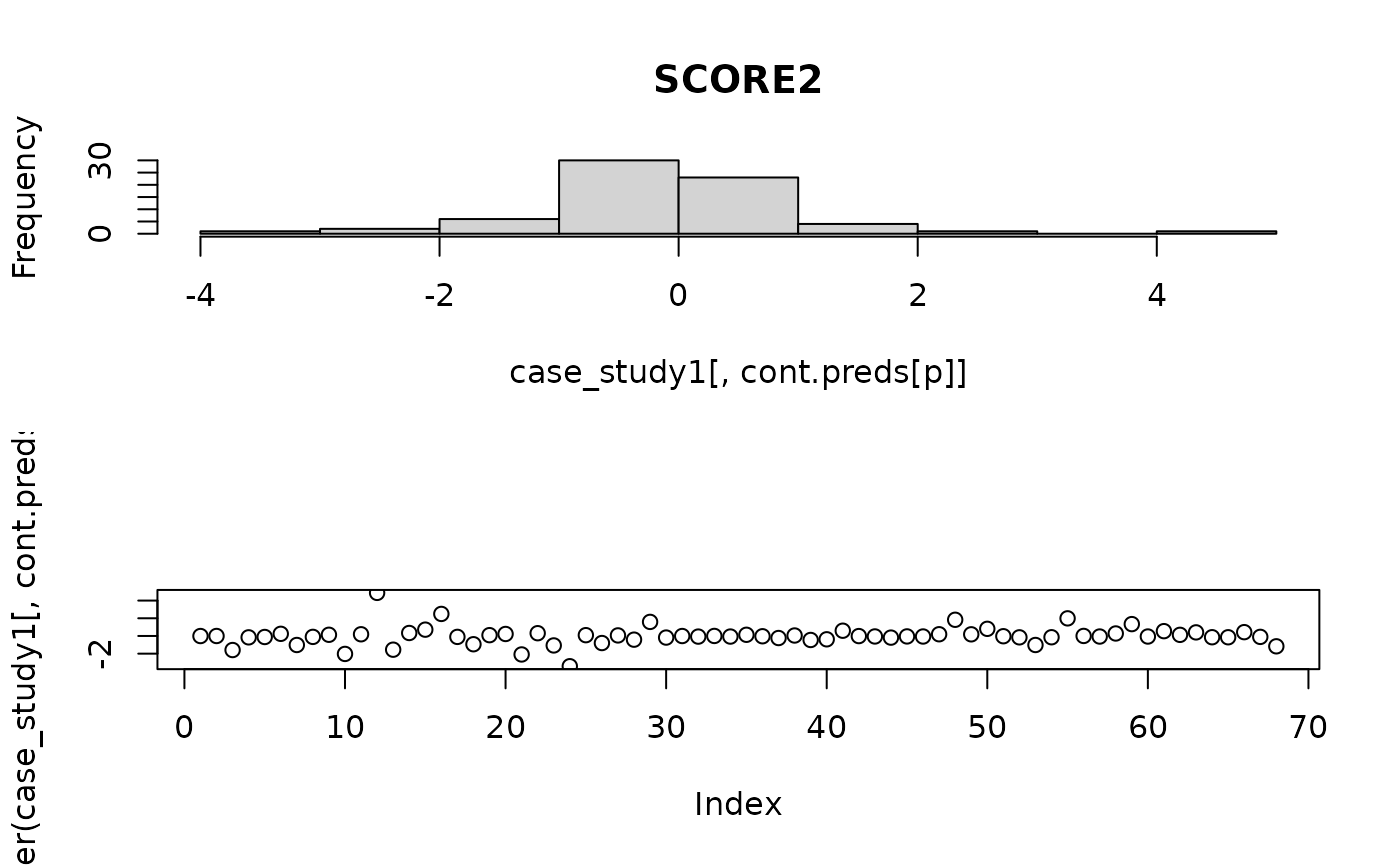
)It is useful to have a look at the distribution of the continuous predictors to ensure they are well distributed (following the transformation above).
for(p in 1:length(cont.preds)){
par(mfrow=c(2,1))
 hist(case_study1[,cont.preds[p]],main=cont.preds[p])
 plot(jitter(case_study1[,cont.preds[p]]))
 }
Full subsets GAMM analysis
Both abundance and biomass data were modelled using a tweedie distribution, passed to FFSgam via a list.
resp.vars.fams <- list(
Herbivore.abundance = tw(),
Invertivore.abundance = tw(),
Piscivore.abundance = tw(),
Planktivore.abundance = tw(),
Herbivore.biomass = tw(),
Invertivore.biomass = tw(),
Piscivore.biomass = tw(),
Planktivore.biomass = tw()
)
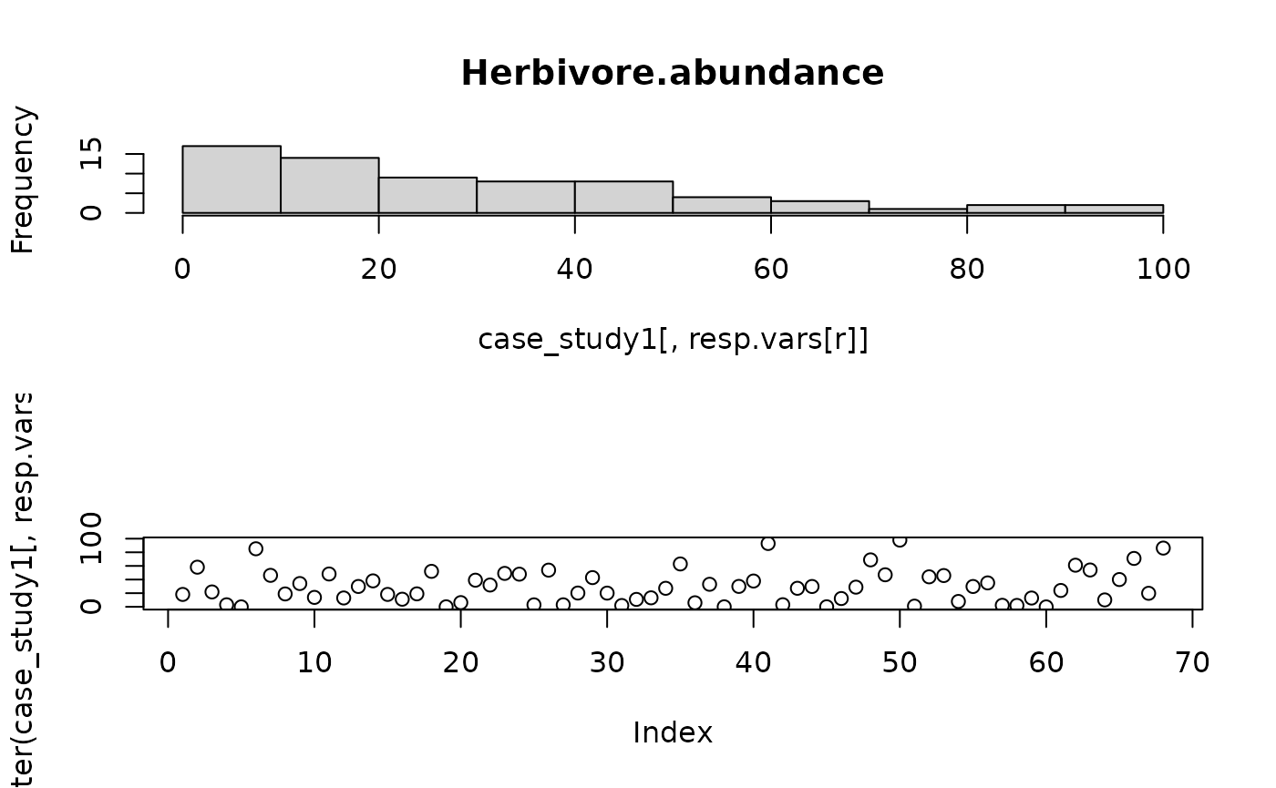
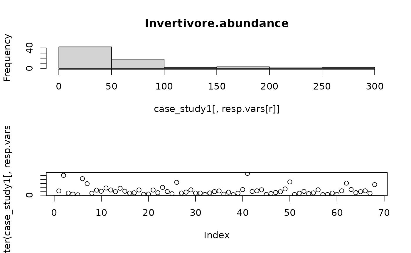
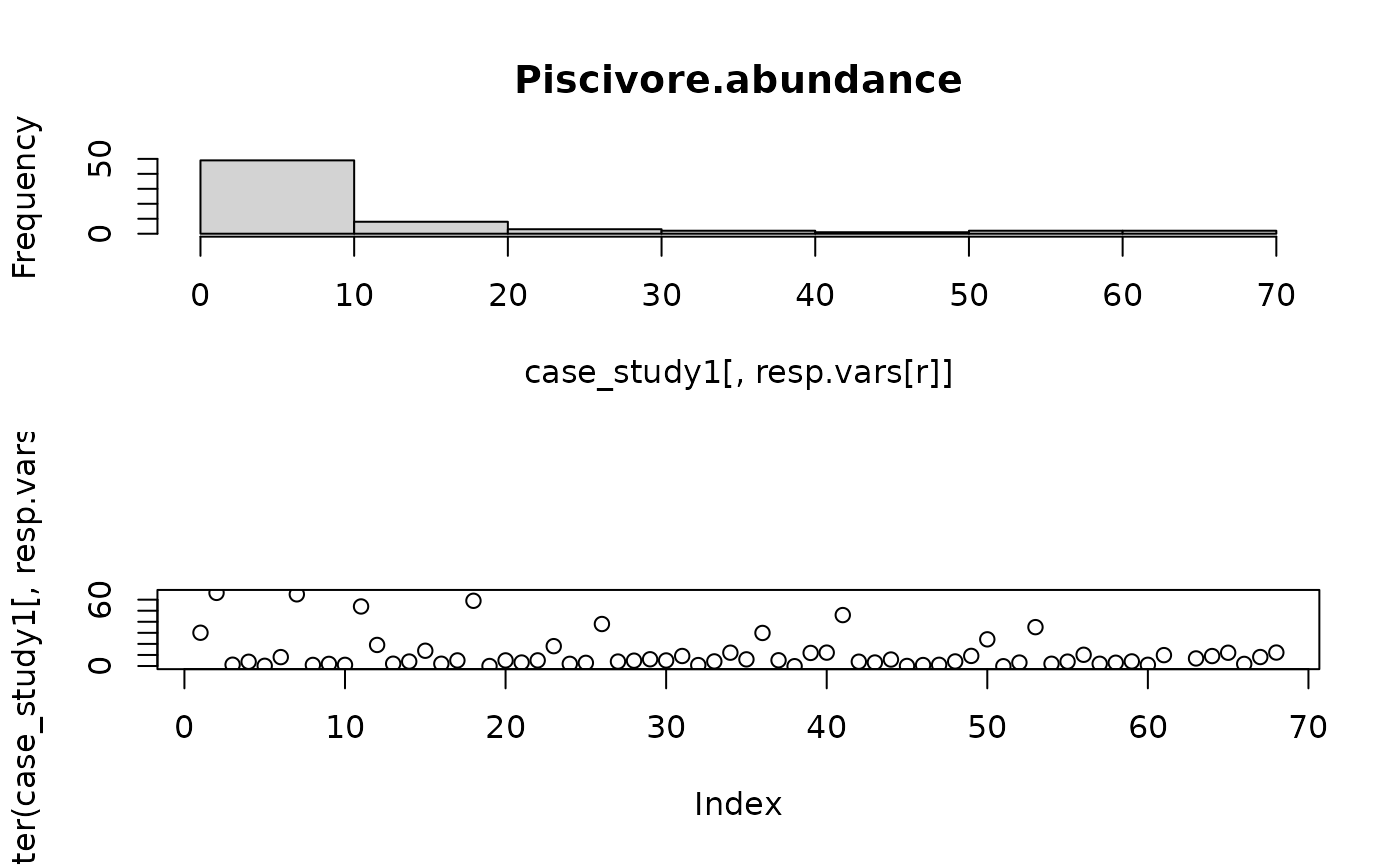
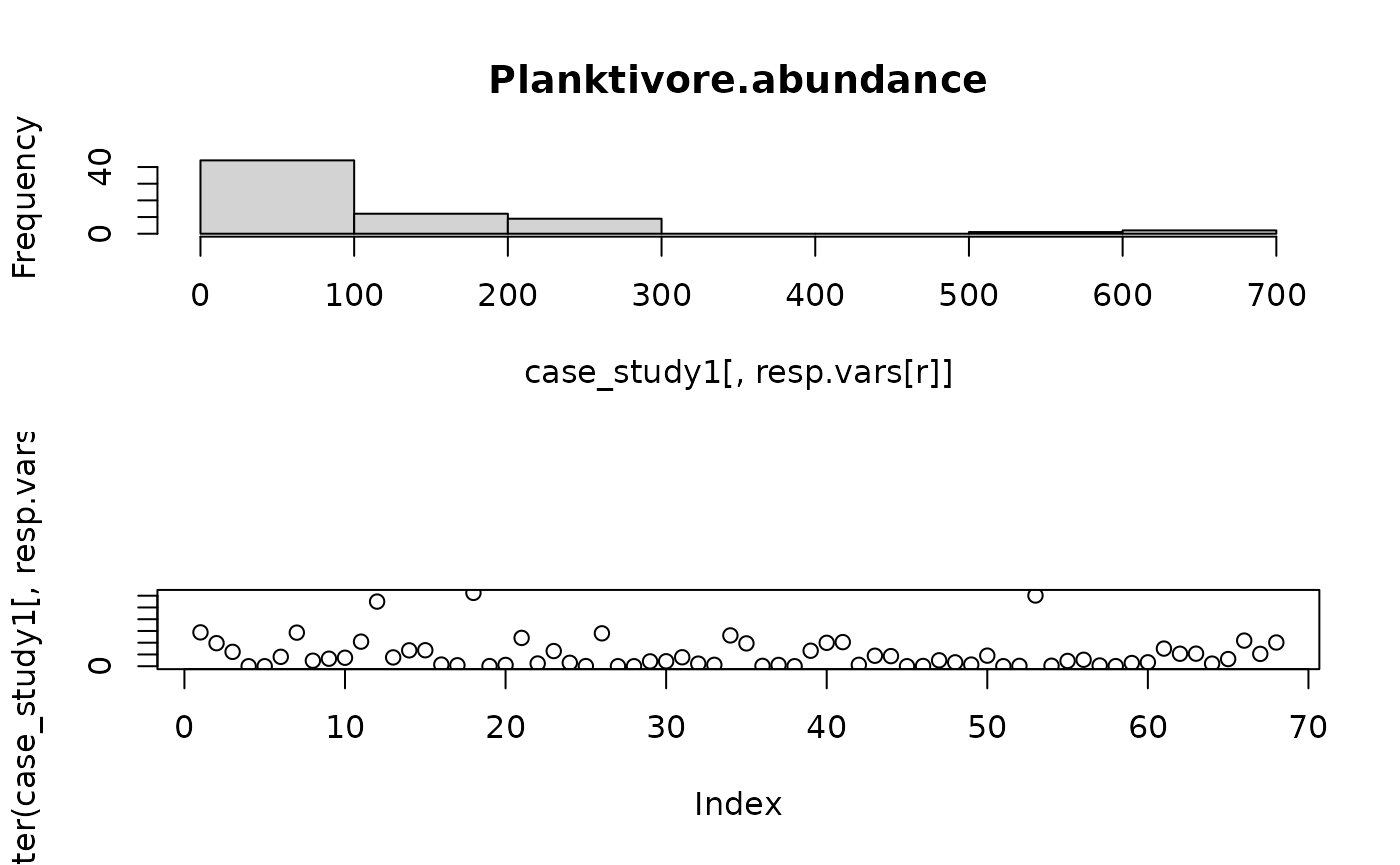
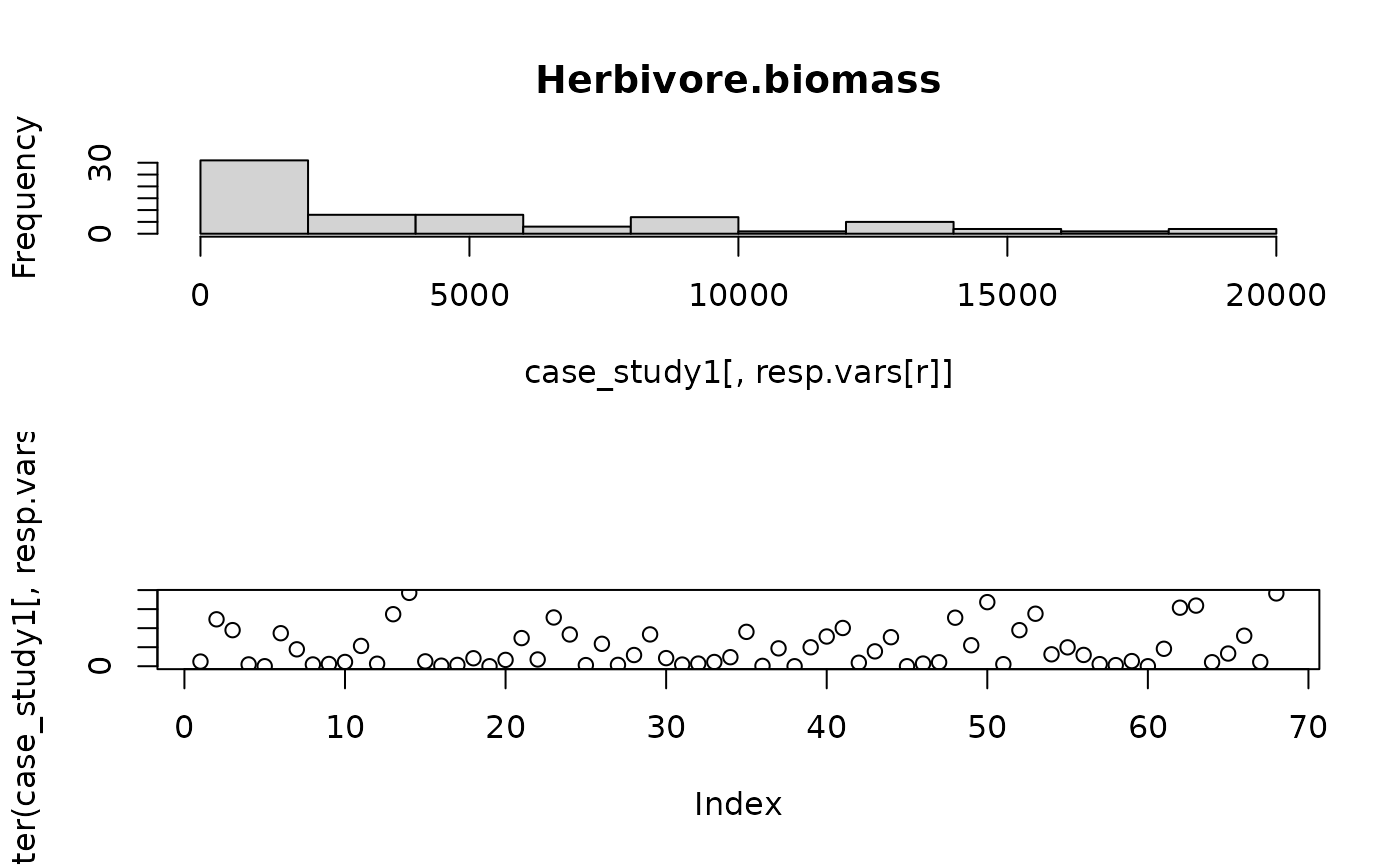
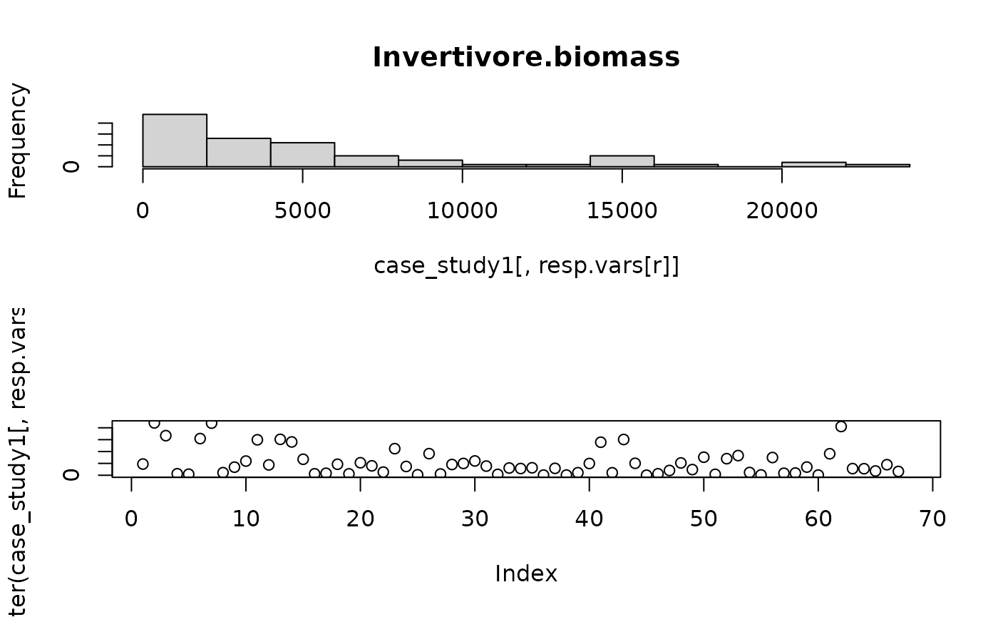
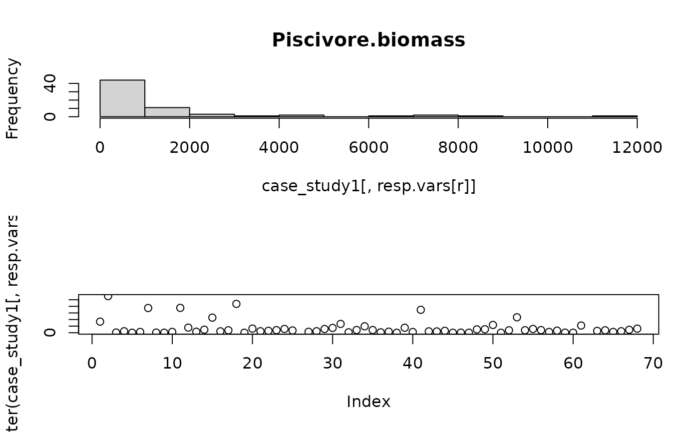
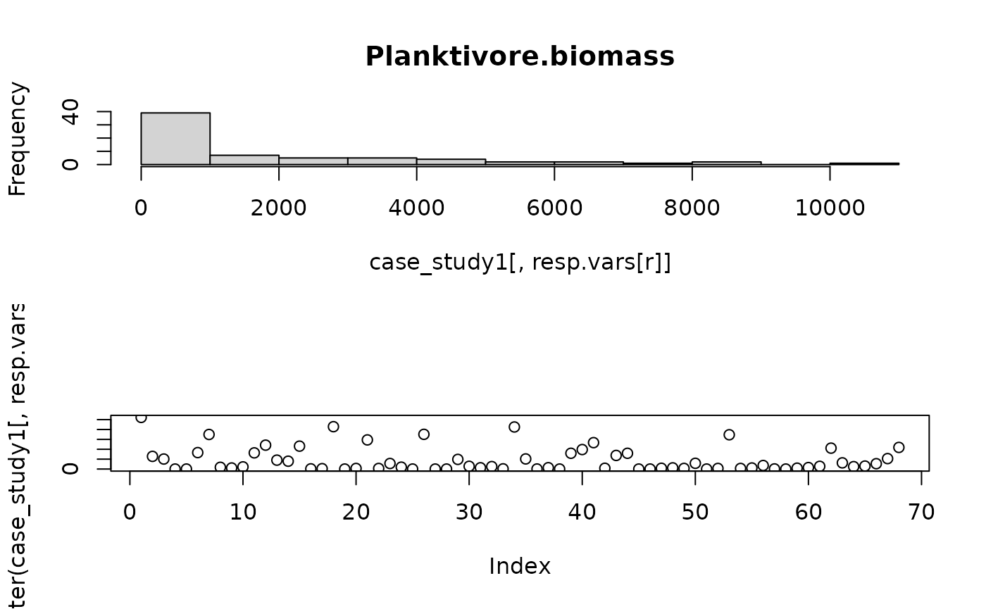
resp.vars <- names(resp.vars.fams)It is always a good idea to look at the response variables, and make sure they suit the distribution.
for(r in 1:length(resp.vars)){
par(mfrow=c(2,1))
 hist(case_study1[,resp.vars[r]],main=resp.vars[r])
 plot(jitter(case_study1[,resp.vars[r]]))
}
 The models are then implemented via a call to gam (mgcv) with the random
effect of site included using the bs=’re’ specification. Smoothers to
both square-route surface area of the patch reef as well as depth were
included in all models (and as part of the null model) via the
null.terms argument of the full subsets gam function.
The models are then implemented via a call to gam (mgcv) with the random
effect of site included using the bs=’re’ specification. Smoothers to
both square-route surface area of the patch reef as well as depth were
included in all models (and as part of the null model) via the
null.terms argument of the full subsets gam function.
Given the complexity of the null model, the maximum number of additional predictors were limited to only an additional two terms (max.predictors=2) and k was limited to 3 to enforce strictly monotonic relationships.
out.all <- list()
var.imp <- list()
fss.all <- list()

for (rv in resp.vars) {

  use.dat <- na.omit(case_study1[, c(null.vars, cont.preds, cat.preds, rv)])
  use.dat$response <- use.dat[, rv]

  base.mod <- gam(
    response ~
      s(complexity, k = 4, bs = "cr") +
      s(SQRTSA, k = 4, bs = "cr") +
      s(site, bs = "re"),
    family = tw(),
    data = use.dat
  )

  model.set <- generate_model_set(
    use.dat = use.dat,
    test.fit = base.mod,
    max.predictors = 2,
    k = 3,
    pred.vars.cont = cont.preds,
    pred.vars.fact = cat.preds,
    null.terms = "s(SQRTSA,bs='cr',k=3)+s(site,bs='re')+s(depth,bs='cr',k=3)"
  )

  out.list <- fit_model_set(model.set, parallel = FALSE)

  var.imp[[rv]] <- out.list$variable.importance$aic$variable.weights.raw
  out.all[[rv]] <- out.list$mod.data.out
  fss.all[[rv]] <- out.list
}
## | | | 0% | |== | 4% | |===== | 7% | |======== | 11% | |========== | 14% | |============ | 18% | |=============== | 21% | |================== | 25% | |==================== | 29% | |====================== | 32% | |========================= | 36% | |============================ | 39% | |============================== | 43% | |================================ | 46% | |=================================== | 50% | |====================================== | 54% | |======================================== | 57% | |========================================== | 61% | |============================================= | 64% | |================================================ | 68% | |================================================== | 71% | |==================================================== | 75% | |======================================================= | 79% | |========================================================== | 82% | |============================================================ | 86% | |============================================================== | 89% | |================================================================= | 93% | |==================================================================== | 96% | |======================================================================| 100%
## | | | 0% | |== | 4% | |===== | 7% | |======== | 11% | |========== | 14% | |============ | 18% | |=============== | 21% | |================== | 25% | |==================== | 29% | |====================== | 32% | |========================= | 36% | |============================ | 39% | |============================== | 43% | |================================ | 46% | |=================================== | 50% | |====================================== | 54% | |======================================== | 57% | |========================================== | 61% | |============================================= | 64% | |================================================ | 68% | |================================================== | 71% | |==================================================== | 75% | |======================================================= | 79% | |========================================================== | 82% | |============================================================ | 86% | |============================================================== | 89% | |================================================================= | 93% | |==================================================================== | 96% | |======================================================================| 100%
## | | | 0% | |== | 4% | |===== | 7% | |======== | 11% | |========== | 14% | |============ | 18% | |=============== | 21% | |================== | 25% | |==================== | 29% | |====================== | 32% | |========================= | 36% | |============================ | 39% | |============================== | 43% | |================================ | 46% | |=================================== | 50% | |====================================== | 54% | |======================================== | 57% | |========================================== | 61% | |============================================= | 64% | |================================================ | 68% | |================================================== | 71% | |==================================================== | 75% | |======================================================= | 79% | |========================================================== | 82% | |============================================================ | 86% | |============================================================== | 89% | |================================================================= | 93% | |==================================================================== | 96% | |======================================================================| 100%
## | | | 0% | |== | 4% | |===== | 7% | |======== | 11% | |========== | 14% | |============ | 18% | |=============== | 21% | |================== | 25% | |==================== | 29% | |====================== | 32% | |========================= | 36% | |============================ | 39% | |============================== | 43% | |================================ | 46% | |=================================== | 50% | |====================================== | 54% | |======================================== | 57% | |========================================== | 61% | |============================================= | 64% | |================================================ | 68% | |================================================== | 71% | |==================================================== | 75% | |======================================================= | 79% | |========================================================== | 82% | |============================================================ | 86% | |============================================================== | 89% | |================================================================= | 93% | |==================================================================== | 96% | |======================================================================| 100%
## | | | 0% | |== | 4% | |===== | 7% | |======== | 11% | |========== | 14% | |============ | 18% | |=============== | 21% | |================== | 25% | |==================== | 29% | |====================== | 32% | |========================= | 36% | |============================ | 39% | |============================== | 43% | |================================ | 46% | |=================================== | 50% | |====================================== | 54% | |======================================== | 57% | |========================================== | 61% | |============================================= | 64% | |================================================ | 68% | |================================================== | 71% | |==================================================== | 75% | |======================================================= | 79% | |========================================================== | 82% | |============================================================ | 86% | |============================================================== | 89% | |================================================================= | 93% | |==================================================================== | 96% | |======================================================================| 100%
## | | | 0% | |== | 4% | |===== | 7% | |======== | 11% | |========== | 14% | |============ | 18% | |=============== | 21% | |================== | 25% | |==================== | 29% | |====================== | 32% | |========================= | 36% | |============================ | 39% | |============================== | 43% | |================================ | 46% | |=================================== | 50% | |====================================== | 54% | |======================================== | 57% | |========================================== | 61% | |============================================= | 64% | |================================================ | 68% | |================================================== | 71% | |==================================================== | 75% | |======================================================= | 79% | |========================================================== | 82% | |============================================================ | 86% | |============================================================== | 89% | |================================================================= | 93% | |==================================================================== | 96% | |======================================================================| 100%
## | | | 0% | |== | 4% | |===== | 7% | |======== | 11% | |========== | 14% | |============ | 18% | |=============== | 21% | |================== | 25% | |==================== | 29% | |====================== | 32% | |========================= | 36% | |============================ | 39% | |============================== | 43% | |================================ | 46% | |=================================== | 50% | |====================================== | 54% | |======================================== | 57% | |========================================== | 61% | |============================================= | 64% | |================================================ | 68% | |================================================== | 71% | |==================================================== | 75% | |======================================================= | 79% | |========================================================== | 82% | |============================================================ | 86% | |============================================================== | 89% | |================================================================= | 93% | |==================================================================== | 96% | |======================================================================| 100%
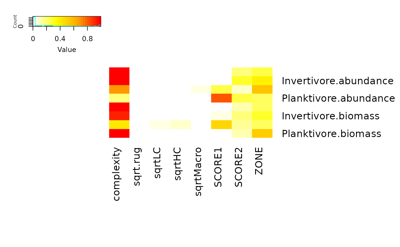
## | | | 0% | |== | 4% | |===== | 7% | |======== | 11% | |========== | 14% | |============ | 18% | |=============== | 21% | |================== | 25% | |==================== | 29% | |====================== | 32% | |========================= | 36% | |============================ | 39% | |============================== | 43% | |================================ | 46% | |=================================== | 50% | |====================================== | 54% | |======================================== | 57% | |========================================== | 61% | |============================================= | 64% | |================================================ | 68% | |================================================== | 71% | |==================================================== | 75% | |======================================================= | 79% | |========================================================== | 82% | |============================================================ | 86% | |============================================================== | 89% | |================================================================= | 93% | |==================================================================== | 96% | |======================================================================| 100%Variable importance
all.var.imp <- do.call(rbind, var.imp)

heatmap.2(
  all.var.imp,
  dendrogram = "none",
  Rowv = FALSE,
  Colv = FALSE,
  col = colorRampPalette(c("white", "yellow", "orange", "red"))(30),
  trace = "none",
  margins = c(12, 14),
  key.title = ""
)
Top model table
all.models <- imap_dfr(
  out.all,
  ~ .x %>% mutate(response = .y)
)

top.models <- all.models %>%
  group_by(response) %>%
  mutate(delta_AICc = AICc - min(AICc, na.rm = TRUE)) %>%
  filter(delta_AICc <= 2) %>%
  arrange(response, AICc) %>%
  ungroup() |>
  select(
    response,
    modname,
    edf,
    AICc,
    delta_AICc,
    wi.AICc)
knitr::kable(
  top.models,
  digits = 3,
  caption = "Top FSSgam models within ΔAICc ≤ 2, ordered best to worst within each response"
)| response | modname | edf | AICc | delta_AICc | wi.AICc |
|---|---|---|---|---|---|
| Herbivore.abundance | complexity | 6.22 | 517.577 | 0.000 | 0.545 |
| Herbivore.biomass | complexity | 6.20 | 1193.357 | 0.000 | 0.648 |
| Invertivore.abundance | complexity | 8.58 | 609.964 | 0.000 | 0.318 |
| Invertivore.abundance | complexity+ZONE | 9.04 | 610.091 | 0.127 | 0.298 |
| Invertivore.abundance | complexity+SCORE2 | 9.35 | 610.185 | 0.221 | 0.284 |
| Invertivore.biomass | complexity | 6.42 | 1236.194 | 0.000 | 0.490 |
| Piscivore.abundance | complexity+ZONE | 6.01 | 457.410 | 0.000 | 0.241 |
| Piscivore.abundance | complexity | 5.64 | 457.424 | 0.014 | 0.239 |
| Piscivore.abundance | complexity.by.ZONE+ZONE | 7.00 | 458.609 | 1.199 | 0.132 |
| Piscivore.abundance | SCORE1.by.ZONE+ZONE | 7.86 | 458.616 | 1.206 | 0.132 |
| Piscivore.biomass | SCORE1 | 5.05 | 1023.292 | 0.000 | 0.290 |
| Piscivore.biomass | complexity | 5.00 | 1023.699 | 0.407 | 0.236 |
| Planktivore.abundance | SCORE1 | 6.72 | 686.784 | 0.000 | 0.453 |
| Planktivore.biomass | complexity+ZONE | 9.65 | 1011.661 | 0.000 | 0.471 |
| Planktivore.biomass | complexity | 9.31 | 1012.086 | 0.425 | 0.381 |
Predictor correlations
It can also be a good idea to check your predictor correlations.
knitr::kable(
  model.set$predictor.correlations,
  digits = 2,
  caption = "Predictor correlations",
  row.names = FALSE
)| complexity | sqrt.rug | sqrtLC | sqrtHC | sqrtMacro | SCORE1 | SCORE2 | ZONE |
|---|---|---|---|---|---|---|---|
| 1.00 | 0.75 | 0.51 | 0.32 | -0.62 | 0.89 | -0.12 | 0.01 |
| 0.75 | 1.00 | 0.33 | 0.40 | -0.58 | 0.85 | 0.10 | 0.09 |
| 0.51 | 0.33 | 1.00 | -0.07 | -0.37 | 0.57 | -0.66 | 0.14 |
| 0.32 | 0.40 | -0.07 | 1.00 | -0.48 | 0.48 | 0.73 | 0.01 |
| -0.62 | -0.58 | -0.37 | -0.48 | 1.00 | -0.82 | -0.15 | 0.03 |
| 0.89 | 0.85 | 0.57 | 0.48 | -0.82 | 1.00 | 0.00 | 0.07 |
| -0.12 | 0.10 | -0.66 | 0.73 | -0.15 | 0.00 | 1.00 | 0.10 |
| 0.01 | 0.09 | 0.14 | 0.01 | 0.03 | 0.07 | 0.10 | 1.00 |
Pretty plots
case_study1 <- case_study1 |>
  mutate(ZONE=factor(ZONE))
zones=levels(case_study1$ZONE)
par(mfcol=c(4,2),mar=c(4,4,0.5,0.5),oma=c(2,0.5,0.5,0.5),bty="l")
for(r in 1:length(resp.vars)){
      tab.r<-out.all[[resp.vars[r]]] |>
        arrange(desc(wi.AICc))
      top.mods.r<-tab.r[1,]
      mod.r.m<-as.character(top.mods.r[1,"modname"])
      mod.m<-fss.all[[resp.vars[r]]]$success.models[[mod.r.m]]
      mod.vars<-unique(unlist(strsplit(unlist(strsplit(mod.r.m,split="+",fixed=T)),
                       split=".by.")))
      # which continuous predictor is the variable included?
      plot.var<-as.character(na.omit(mod.vars[match(cont.preds,mod.vars)]))
      # plot that variables, with symbol colours for zone
      plot(case_study1[,plot.var],case_study1[,resp.vars[r]],pch=16,
         ylab=resp.vars[r],xlab=plot.var,col=case_study1$ZONE)
      legend("topleft",legend=paste("(",LETTERS[r],")",sep=""),
             bty="n")
      range.v<-range(case_study1[,plot.var])
      seq.v<-seq(range.v[1],range.v[2],length=20)
      newdat.list<-list(seq.v,# across the range of the included variable
                       mean(use.dat$depth), # for a median depth
                       mean(use.dat$SQRTSA),# for a median SQRTSA
                       "MANGROVE", # pick the first site, except don't predict on
                               # this by setting terms=c(plot.var,"ZONE")
                       zones)  # for each zone
      names(newdat.list)<-c(plot.var,"depth","SQRTSA","site","ZONE")
      pred.vals<-predict(mod.m,newdata=expand.grid(newdat.list),
                     type="response",se=T,exclude=c("site","SQRTSA","depth"))
      for(z in 1:length(zones)){
       zone.index<-which(expand.grid(newdat.list)$ZONE==zones[z])
       lines(seq.v,pred.vals$fit[zone.index],col=z)
       lines(seq.v,pred.vals$fit[zone.index]+pred.vals$se[zone.index]*1.96,lty=3,col=z)
       lines(seq.v,pred.vals$fit[zone.index]-pred.vals$se[zone.index]*1.96,lty=3,col=z)}
}
legend("bottom",legend= zones,bty="n",ncol=2,col=c(1,2),pch=c(16,16),
   inset=-0.61,xpd=NA,cex=.8)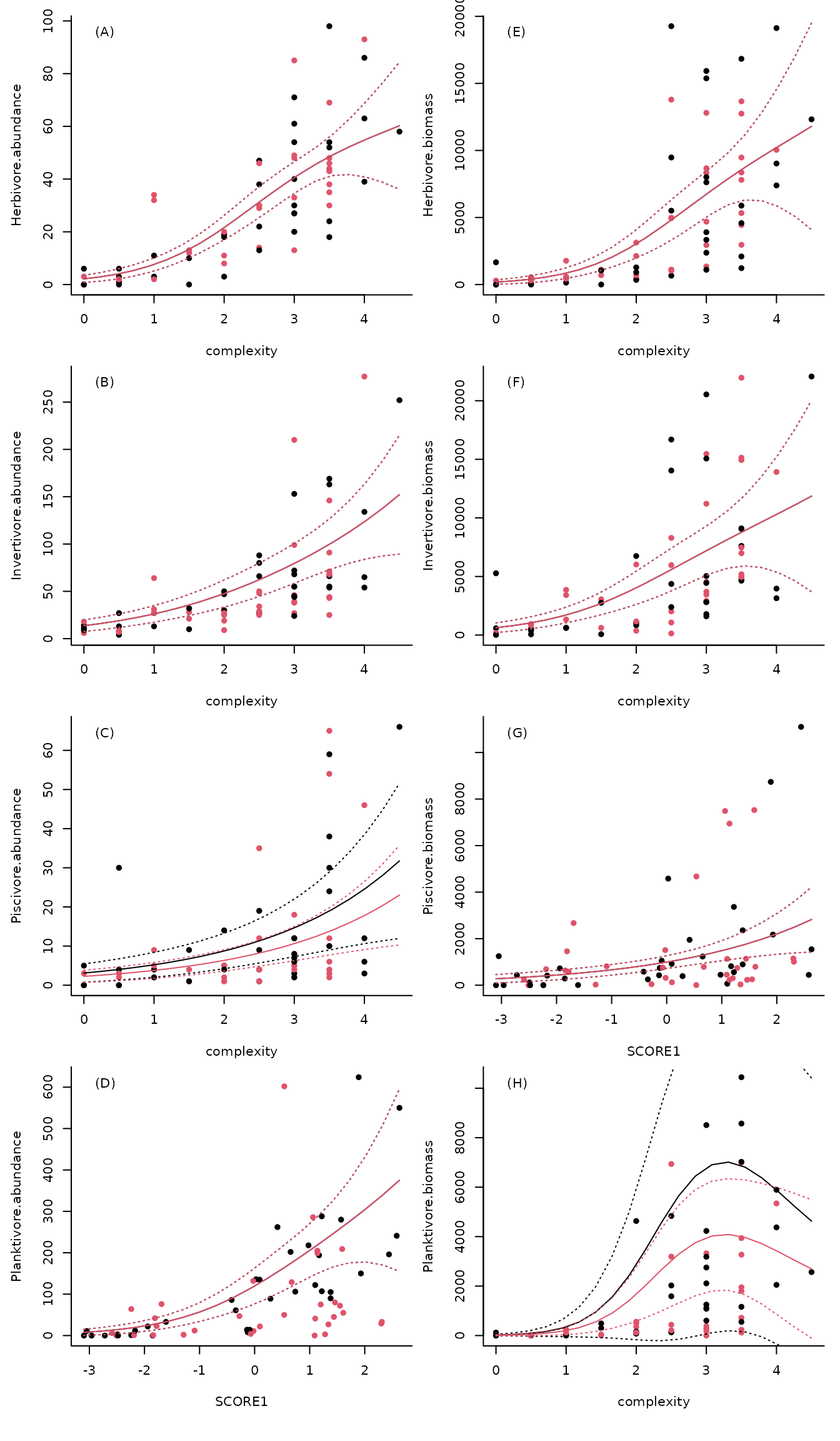
Results and discussion
Seascape measures of patch reef complexity were generally the best predictor of both fish abundance and biomass (see the model comparison table above). Fish abundance and biomass were low on reefs with no relief and were higher on structurally complex reefs (see the predictor plots above). These findings are consistent with other studies that show measures of seascape complexity are positively correlated with fish abundance, and often outperform other measures of complexity (Wilson et al. 2007; Collins et al. 2016). The results generally support the original findings of Wilson et al. (2012) that there are strong relationships with habitat and only weak evidence for an effect of the zoning status. However, here we were able to tease apart the influence of correlated habitat variables. For example, the revised analysis found herbivore abundance was positively correlated with complexity, which is similar to recent studies at Ningaloo that also found abundance of these fish is not closely related to macroalgal cover (Wilson et al. 2014) and is better explained by reef structure (Downie et al. 2013). Conversely, Wilson et al. (2012) identified scores from principal component 1 as the best predictor of herbivore abundances, which inferred a positive effect of both rugosity and complexity and a negative effect of macroalgal cover.
Interestingly, the abundance of planktivores and piscivores was positively related to scores from principal component 1 (see the variable importance heatmap and predictor plots above), suggesting summarised metrics of habitat from PCA may still be relevant to some components of the fish assemblage. A habitat descriptor that incorporates multiple correlated factors may be more important if there is a diverse array of habitat associations among fish within a trophic guild. For example, the planktivores include small bodied damselfish that have close associations with complex corals (Coker et al. 2014), cardinalfish that are often found in caves or branching corals (Marnane and Bellwood 2002), and larger fish that are likely transient and more associated with seascape measures of habitat (Friedlander and Parrish 1998). As large bodied fish also typically contribute more to community biomass than their small counterparts (Ackerman and Bellwood 2000) it is not surprising that planktivore biomass is more closely aligned with seascape complexity than other measures of habitat.
Overall the results of the revised analysis are similar to those from the original study based on the use of data-reduction via PCA. However, by including the underlying habitat information, the new analysis provides a clearer picture of which elements of the benthic assemblage are most important to fish. This additional information is useful for building scientific hypotheses and parametric functional models for how such fishes may be influenced by changes in habitat (such as is expected due to ocean warming and climate change, see (Pratchett et al. 2015)), as well as informing which elements of the habitat should be a focus for management targets.
This example demonstrates how full subsets GAMMs can be used to synthesise drivers across multiple response variables in ecological datasets.